


Game engines do most of their shading work per-pixel or per-fragment. But there is another alternative that has been popular in film for decades: object space shading. Pixar’s RenderMan®, the most well-known renderer for Computer Graphics, uses the Reyes rendering method, which is an object space shading method.
This blog looks at an object space shading method that works on Direct3D® 11 class hardware. In particular, we’ll be looking at texture space shading, which uses the texture parameterization of the model. Shading in object space means we have already decoupled the shading rate from pixels, and it’s also easy to decouple in time. We’ve used these decouplings to find ways to improve performance, but we’ll also discuss some future possibilities in this space.
Texture Space Shading
When most people hear the term “texture space shading” they generally think of rasterizing geometry in texture space. There are two difficulties with that kind of approach: visibility and choosing the right resolution. Rasterizing in texture space means you don’t have visibility information from the camera view, and end up shading texels that aren’t visible. Also, your resolution choices are limited, as you can only rasterize at one resolution at a time.
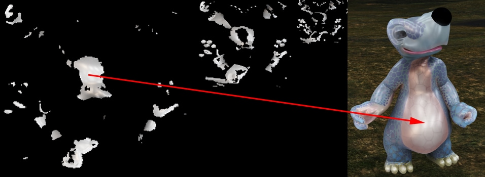
Resolution choice is important because it drives your total shading cost. Each mipmap level costs an additional 4× shading cost. So if you need 512×512 to match pixel rate for one part of an object and 1024×1024 for another part, but you can only pick one, which do you pick? If you pick 512×512, part of the object will be under sampled. If you pick 1024×1024, part of your object will cost 4× as much as needed. That increases with every level you span. If you have an object that spans 4 mipmap levels, for example, you can increase shading cost by up to 64× to hit a particular resolution target for the whole object! The following image shows just a few levels of a single character’s texture access for the given view, (after early depth rejection has been applied), to give you an idea of just how much waste there can be when not selecting the right resolution in texture space shading.
So let’s try a different approach. Instead, we will rasterize in screen space (from the camera view), and instead of shading, we just record the texels we need as shading work. This is why we chose the term “texel shading”. Since we are rasterizing from the camera view, we get the two pieces of information that aren’t normally available in texture space methods – visibility after early depth test, and the screen space derivative for selecting the mipmap level. The work itself are the texels.
How Texel Shading Works
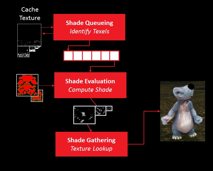
At a high level, the process is as follows:
- Render the model, recording the texels required.
- Shade the texels, writing them to a texture map of results.
- Lookup results while rendering the model a second time.
Note that texel shading can be selectively applied on a per-object, or even per-fragment basis. The fragment-level choice happens at the time of the first geometry pass, so it still incurs additional cost of other stages, but it allows for fall backs to standard forward rendering. It also also allows you to split shading work between texel shading and pixel shading.
There are a few details on how this is done that I will just mention here, but hopefully you have a chance to read the Eurographics short paper on the topic to get a better idea.
One bit of information to know, is that we actually shade 8×8 tiles of texels. We have a sort of cache that has one entry per tile that we use to eliminate redundant tile shades, as well as age tracking for techniques that use shades from previous frames.
The second, is that we need to interpolate vertex attributes in the compute shader. To do so, we have a map we call the “triangle index texture” that we use to identify which triangle we need to shade a particular texel.
The Drawbacks
This alone gives you no benefit. In fact, it incurs additional cost in a few different ways:
- Adds an additional geometry pass, although it may be combined with another geometry pass, or combined with the final pass of the previous frame.
- Shade count starts higher. In our experiments, it’s 20% to 100% more shades, depending on the model. One cause is that we choose resolutions conservatively to at least match pixel rate. This is also because we actually operate on 8×8 tiles, so some texels are shaded when only a subset of the 8×8 texels are visible and at the right resolution. Note I used the term “start”. That’s because we’ll look at ways to reduce this in the next section.
- The overhead of shading in compute. Vertex operations get pushed to per-texel operations. This is why it’s important to consider using preskinned vertices. You must also compute barycentrics and interpolation in shader code yourself. There’s actually untapped potential here as well – with compute, you have explicit access to neighbor information and the possibility of sharing some shading cost across the texel tile.
- Memory cost. Our method requires an allocation of enough texture memory to store shaded results and the triangle index texture at a “high enough” resolution. This is an area for future research.
- Filtering issues. We only experimented with bilinear-point filtering (picking one resolution, bilinear filter within that mipmap level). This is not necessarily good enough for a final shade. In fact, it may be possible to do much more intelligent filtering that turns this into an advantage. In the end, though, anything done in texture space needs to go through texture filtering, which is far from ideal.
Advantages and Potential
However, once you have an object-space rendered like this, new options open up. I’ll list several of them in this section. The first two, and a bit of the third, are what we’ve tried so far. The rest are what we think is worth trying in the future.
- Skip frames. Because the shading occurs in object space, it’s easier to change the temporal shading rate. Our implementation uses a cache of how old shades are, and reuses shades from previous frames, if not too old.
- Variable and multi-rate shading. There’s no reason why the mipmap level choice needs to match pixel rate – you can go higher for better shader antialiasing, or lower for much reduced shading rate in lower-variance regions, and this choice can be made on a per-fragment basis. We experimented with biasing the mipmap level on a per-triangle basis by checking the normal variance, and biasing the mipmap level for lighting calculations if the triangle was relatively flat. It’s also possible to actually shade at different rates for the same fragment – in a sense, we did this by only computing lighting in texture space, and doing a texture lookup at fragment rate – but work could have been split up further to compute different parts at different resolutions at the same time.
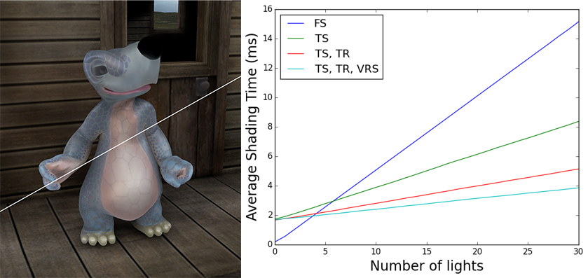
- Decoupled geometry. In a forward renderer, shading efficiency drops quickly with small triangles, and gets worse with Multisampling Anti-Aliasing (MSAA) when samples in a pixel are covered by more than one triangle. Texel shading suffers from neither of these problems, because the shading rate is tied to texel shading rate. We found cases in which texel shading actually outperformed standard forward rendering, before we even got to skipping frames or changing shading rate. But there’s actually more opportunity here. The geometry used for shading can actually be completely different from the triangles that are rasterized in screen space. They can also be different at different mipmap levels. This provides additional opportunity for geometric anti-aliasing that we have not explored.
- Object space, temporal anti-aliasing. Rather than skipping frames to save shading cost (point 2 above), one could instead shade every frame, but average in shades from previous frames as is done in screen space temporal anti-aliasing. Performing this operation in object space avoids some artifacts and workarounds that are necessary for screen-space temporal anti-aliasing.
- Stochastic effects. One attractive feature of object space shading, is that you can reuse shades while applying depth of field or motion blur, without worrying about screenspace artifacts. In fact, this was a major motivation for the Reyes rendering system. There are also methods of finding the right mipmap bias to save shading when rendering a blurred object. This is an item we have not explored.
- Better filtering. Shading in object space, in compute, where we have access to neighboring texels, and in a sort of multi-resolution space, opens up further opportunity for shader filtering. We have not explored this as much as we would like.
- Asyncronous shading and lighting. This was actually the original motivation for this research. Skipping frames is a simpler first step. However, if you have some fall-back system for shades that are not ready in time, you could potentially compute shading completely asynchronously, while still updating the projection of the model on the screen at full rate, using whatever the most recent shade value. This is another area we would like to explore.
- Stereo and other multi-view scenarios. It’s also possible to reuse shading calculations across eyes for VR, with the caveat that many specular effects may not work well. With asynchronous shading or lighting, you could even share shading across a network of individual users looking at the same scene, such as a multi-player game.