


In the above image, on the left side you can see clamping artifacts where much of the flower looks like it has smudges of bright red over it. You can see on the right side the perceptually mapped image which removes these artifacts, but you will notice that the image is also less saturated. This is because contrast was preserved during the perceptual mapping and as a result the image was made slightly darker. The above images are an exaggeration of the artifacts that can come with each mapper, but it shows what kind of trade-offs you may have to make when choosing your gamut mapper.
As part of our FreeSync HDR work, we implemented a clipping gamut mapper since most games have very few out of gamut pixels for any given frame, and it helped to understand how to minimize the perceptual difference between out-of-gamut colors and their mapped in-gamut colors.
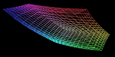
To do this, we needed to work in a color space where the distance between colors is somehow related to how perceptually similar they are. We chose to work in CIELAB since it’s a perceptually uniform color space (check out the first post in the series for more!). We can see below a visualization of a Toshiba monitor’s gamut volume in CIELAB, which is a similar volume to what you would see in sRGB.
We’ll show 2D gamut visualizations, with a lightness axis and a chroma axis as can be seen below:
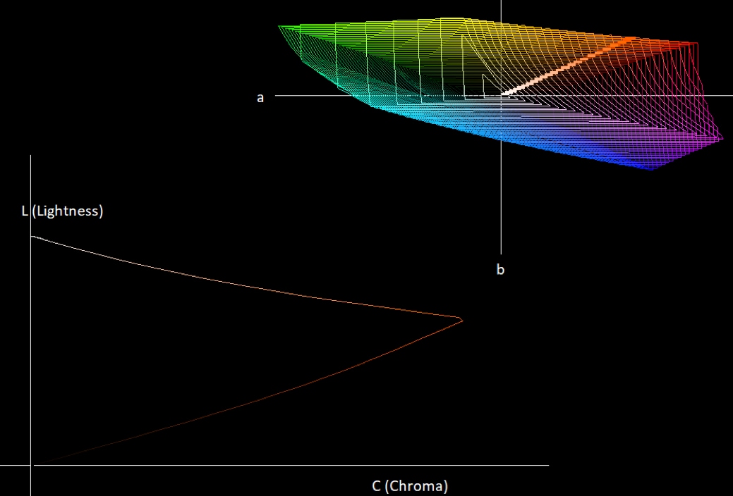
In CIELAB, angles on the a, b plane represent hue, and distance from the origin on the a, b plane represents chroma (check the CIELAB color space). Since our gamut mapper keeps hue constant, to visualize the gamut for some particular hue we can intersect the 3D gamut with a plane which extends to infinity on the lightness axis, and is angled to our hue value on the a, b axis. In the top-right corner of the above visualization, we can see the 3D gamut projected on the a, b plane and a line going through the orange part of the gamut. That line represents the plane that we are intersecting with the 3D gamut to generate the triangle on the bottom left part of the image (the gamut shape for that hue value). For each hue value, we will only be showing the values with positive chroma as done above.
In the gamut mapping problem domain, we have a source gamut which represents the colors in our input image, and we have a target gamut which represents the colors a monitor can display. Throughout this blog post, I will be showing visualizations like the one below of the source and target gamut for some arbitrary hue, with the lightness and chroma axes displayed.
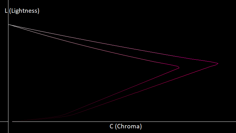
In the above visualization, the highest point on the L axis represents the brightest color that can be displayed by our monitor (its brightness can be queried using FreeSync HDR). In the image above, we can also see the region of colors that are outside the target gamut but inside the source gamut. These are the colors that will need to be mapped on to the target gamut while looking as perceptually similar as possible to the out-of-gamut color. Since CIELAB is perceptually uniform, we use Euclidean distance as a measure of perceptual uniformity. This isn’t a perfect measure of perceptual distance since as the colors get farther away each other, Euclidean distance becomes less accurate, but we found that with some changes in the direction we move our colors, we can get good results.
Gamut Mapping Algorithm
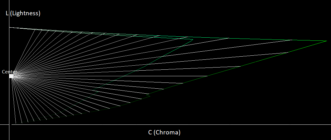
When building a gamut mapper, it’s common to set some color property as unchanging between the source and mapped color, so that we limit the amount of directions we have to move to find a mapped color. For clipping gamut mappers, we found that most research focused on keeping hue constant since changes in hue are more perceptible than changes in lightness or chroma. Chroma is seen as the most changeable color property since we notice differences in chroma less than we do for lightness. Knowing this, we first tried to keep hue and lightness constant, and only change the chromaticity value until the color was in gamut. This however resulted in lots of pixels becoming completely desaturated and we can see exactly why in the visualization below:

In the above image, the yellow line represents the direction the color would travel if we kept lightness and hue constant. As we can see, because of the gamut’s irregular shape, if we keep the hue and lightness constant, we can end up moving very far before we find an in-gamut color. We can also see that if we could modify lightness and move in the direction of the blue line, then we could move down a little on the L axis and find a color that is much closer to our original color. Noticing this, we allowed colors to modify their lightness value and had them move towards the center of the L axis as shown below:
This resulted in much better color preservation from Rec2020 to our monitor’s gamut, but it still has a few issues. For dark colors at the bottom of the gamuts, we can see that they map to a brighter color in the target gamut even though there are closer colors which maintain a similar level of lightness. The same is true for the higher parts of the gamut, where they map downwards too much, reducing lightness, even though there are closer colors with similar levels of lightness.
Finally, we can see that near the target gamut’s tip, there are very few colors which map to it, while the lower parts of the target gamut have a lot more lines which converge to them. This means that the we are mapping colors from the source gamut non-uniformly to the target gamut, causing more color collisions which creates clipping artifacts.
To combat this, we implemented the algorithm in this paper (Masaoka-san et al., 2016) which takes the gamut’s triangle-like shape into account to calculate the direction which colors should move to hit the source gamut. This resulted in smaller distances that colors needed to move to map to the target gamut, while also mapping colors more uniformly. The rest of this section will be going over step-by-step how to implement the gamut mapping paper, and how each step helps improve the algorithm.
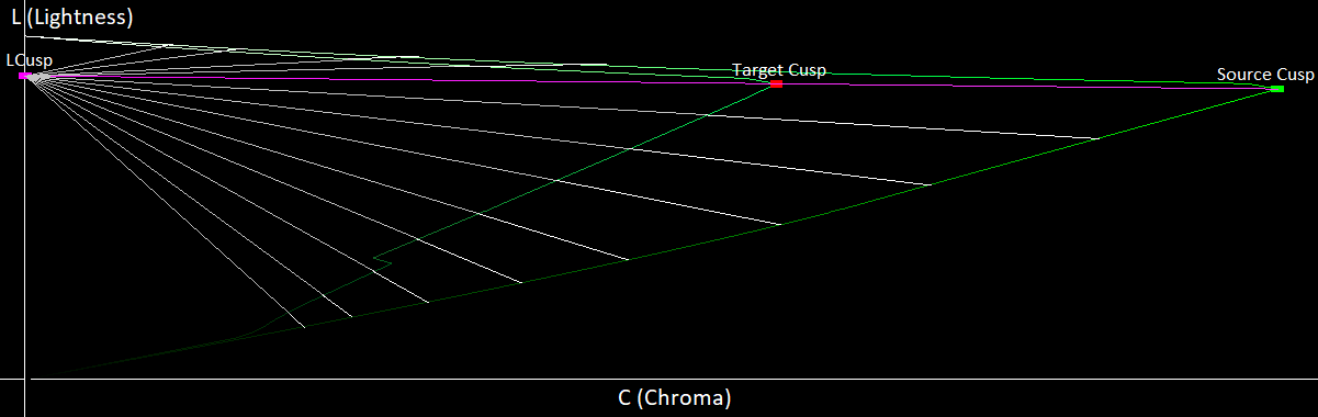
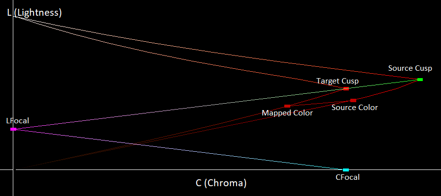
To start implementing this paper, we need to define a few points. We call the gamut cusp the point on a gamut with the highest chroma value for some specified hue (the gamut cusp for the source/target gamut is called the source/target cusp). In the above visualization, the source/target cusps are the farthest points to the right that are in-gamut.
Since the gamut’s shape is triangle-like, we want everything above the gamut’s cusp to map downwards on the gamut and everything below the cusp should map upwards towards the gamut, since those are the paths of smallest Euclidean distance. To get this behavior, we can create a cusp line that passes through the source and target gamut’s cusps and have it intersect the L axis. This will give us a point called LCusp as can be seen in the image below:
If we look in the above image, we can see that the bright colors are better mapped, without such drastic changes in lightness, but the dark colors are still being brightened significantly. To fix this, we want to change the mapping direction for the darker colors to be more horizontal since our eyes are more sensitive to changes in the lightness levels of dark colors. To do this, we check if the cusp line is angled downwards or upwards. If its angled downwards, then we extend it until it intersects the C axis. This point of intersection we call the CFocal as shown below.
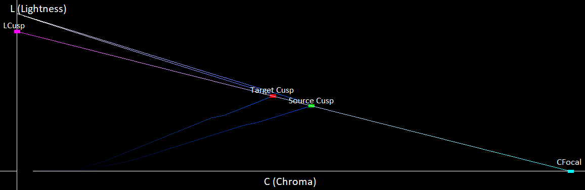
If it’s angled upwards, then we reflect the cusp line at LCusp. Wherever the reflected cusp line intersects the C axis, we call that point CFocal as shown below.
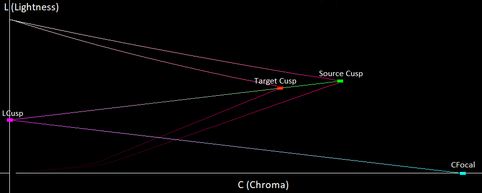
If you look at the triangle connecting CFocal and LCusp, we see that all the dark colors between our two gamuts are inside of this triangle, so when we map these colors, as they get darker we want them to move more horizontally. This can be achieved by mapping them away from CFocal instead of towards LFocal, giving us the following directions that our colors move in:
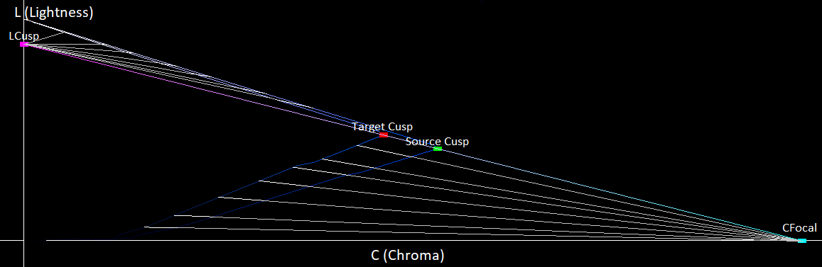
Doing this, our mapping process now better maps dark colors to other dark colors, but it also maps the colors more uniformly onto the target gamut surface since we avoid having surface points which colors from the above and below map to.
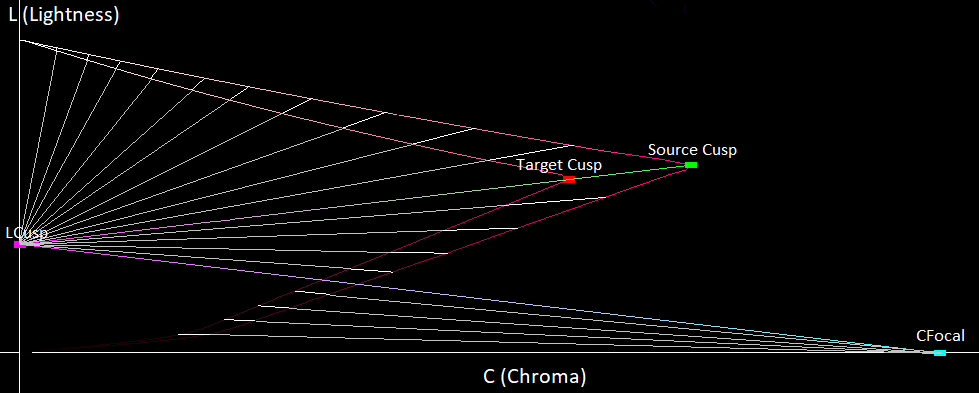
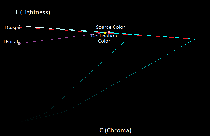
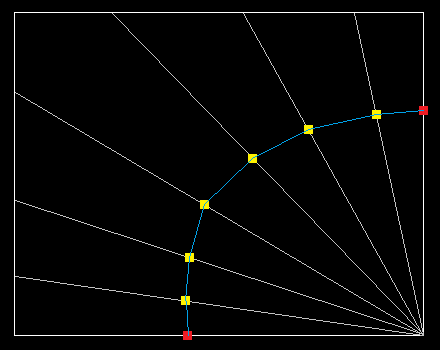
There is one final change we need to make to this mapping process. In the below image, we provide an example of a color that gets significantly desaturated.
It’s a little hard to make out, but the red line represents the line which generates LCusp, while the yellow line is the line from the source color to LCusp. We can see that the source color moves all the way to the destination color, even though there is a much closer desired color that we want it to map too. This happens when the line between the source color and LCusp is almost parallel to the gamut’s surface, making the source color move very far before it intersects the target gamut. This circumstance arises when LCusp is almost at peak lightness like in the image above.
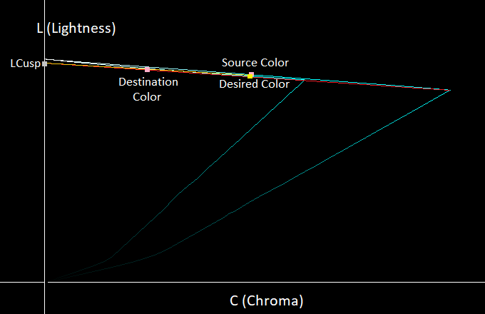
To prevent this, we clamp LCusp to be between a certain range, and we call the new point LFocal. The range was chosen in the paper by finding the values that provide the smallest perceptual difference for each hue angle. If we apply this fix to the above image, we get the below result.
By limiting how high on the L axis LFocal can be, we make sure that bright colors are still mapped downwards and are never mapped upwards, preventing heavy color desaturation. Now we have a derived gamut mapping algorithm as an implementation of the paper (Masaoka-san et al., 2016). When mapping colors in practice, given an out-of-gamut color, we generate the gamut for the color’s hue, and we run the above gamut intersection algorithm. Below we provide a final visualization which brings together all the concepts we have described so far and shows how we map a color in practice.
Generating A Gamut Volume
Now that we know how the gamut mapper itself works, we need to know how to generate the 3d gamut volume so that we can write the above algorithm. To do this, we turned to this paper (Sun, Liu, Li and Zhou, 2014) which generates our gamut boundary at a bunch of constant lightness values in RGB, giving us an approximation of the 3D gamut. The paper notices that on the surface of the RGB cube, if we have a point X with lightness of A and point Y with lightness of B, then on the line between X and Y there exist points with all the lightness values between A and B.
The paper then derives an interpolation formula which finds the point between X and Y with a desired lightness value between A and B. The paper’s formula seemed to find points with different lightness values and we couldn’t get it to work, so we derived our own interpolation formula. Using the fact that the RGB cube’s surface represents the gamut boundary in RGB, the paper derives a formula for generating gamut boundary for a fixed lightness value on the RGB cube’s surface. The algorithm works as follows:
Given a lightness value, we check every edge on the RGB cube to see if our lightness value falls between range of the edge’s endpoints.
If it does, we use our interpolation formula to find the gamut boundary point on that edge.
After doing this for each edge, we get a set of points that we connect to generate a shape. This shape will be a triangle, or a rectangle as can be seen below:
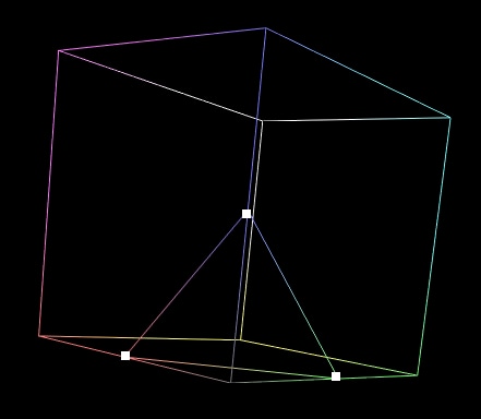
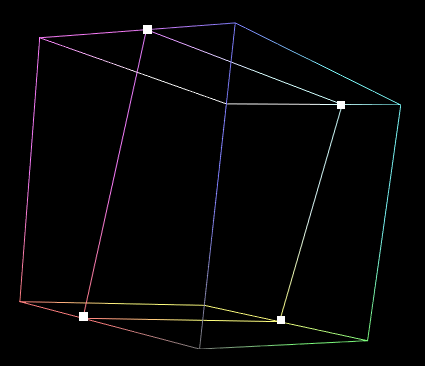
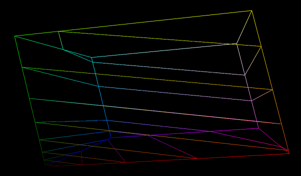
The current generated shape has straight lines connecting each point that go across entire cube faces, but the real gamut boundary may be curved in RGB, and not a straight line. To fix this, we need to better sample the gamut boundary across the cube’s faces, and we do this by generating lines across the cube faces as can be seen in the image below.
The red points above are the points we found previously on the cube’s edges, while the yellow points are the new points we found by sampling more along the cube’s face. We first generate these lines from the corner and we know these lines must intersect the gamut boundary curve since the curve connects continuously between both red points. We then use the interpolation formula on each of the generated lines to find the point with our lightness value, and we connect them as we did above. We do this for every face that our gamut boundary curve touches, giving us more refined gamut boundaries. We then repeat this process for every plane we want to generate, giving us a set of closed curves in RGB that represent gamut boundaries at different lightness values. Below we show a visualization of the gamut boundaries on the RGB cube.
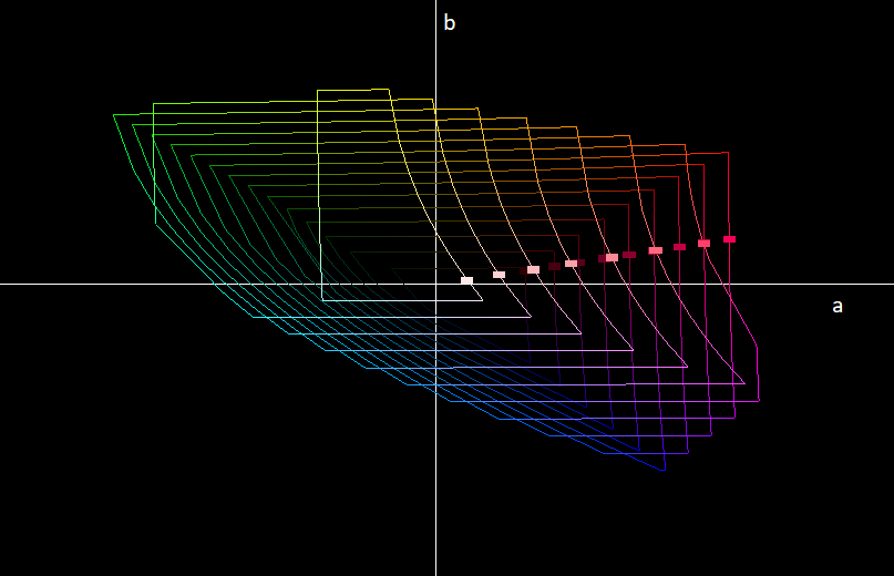
When plotting the above curves in CIELAB space, we get the following result:
When we intersect the color with our gamut, we only need to do the intersection test for the part of the gamut that intersects the hue plane. The squares in the above image represent the intersection points between the gamut boundary planes and the hue plane with positive chroma. If we plot these points such that the horizontal axis is chroma and the vertical axis is lightness, then we get the following:
In the above image we connected the intersection point with each other to generate the gamut shape. The hard edges in the above image are only there for the purposes of this post; our gamut mapper generates many more gamut boundary curves to better sample the gamut shape. We can now easily find the intersection points between our color and the target gamut by intersecting every line segment in the image above.
FreeSync HDR Gamut Mapping
FreeSync HDR reduces display latency by disabling the monitor’s gamut mapper, reducing processing time on the display side. Prior to FreeSync HDR, games would gamut map the frame and send it off to the monitor which would also gamut map the image, resulting in gamut mapping being applied twice. With FreeSync HDR, only the game gamut maps the frame, removing the latency introduced via the display’s gamut mapper. A potential optimization is that most clipping gamut mappers can be reduced to a look-up table (LUT) and games currently reduce other color processing techniques to LUTs such as color grading, tone mapping, etc., that get combined into one final LUT. By combining the color processing LUT with the gamut mapping LUT, we introduce a very small performance cost, while getting the benefit of latency reduction from FreeSync HDR.
Another benefit of FreeSync HDR is that it provides developers with information on the display’s native gamut, allowing developers to fully utilize the display’s color capabilities. Without FreeSync HDR, games can only gamut map from their source gamut to any of the standard color formats that are supported by the player’s monitor. For example, a game can render the world in Rec2020 and try to map that to an SDR monitor that outputs in Rec709.
The problem is that most displays have non-standard native gamuts that might be larger than Rec709, but smaller than Rec2020. So, if we naively map from Rec2020 to Rec709, we will potentially be mapping to colors that can’t be displayed by our monitor, reducing the potential quality of our image. By using FreeSync HDR, the developer knows the monitor’s native gamut and can ensure that the mapping algorithm only maps colors outside of this gamut, making the algorithm display higher quality images.
Lastly, FreeSync HDR gives the developer the choice of which gamut mapping algorithm to use that best fits the content the developer wants to display. For example, if only a few colors are out of gamut for any given frame, the developer will want to use a clipping algorithm since it preserves the look of the game at a low processing cost. If the game instead has very many colors out-of-gamut, the developer can choose to implement a perceptual gamut mapper that better preserves the look of the image.
Prior to FreeSync HDR, the developer would apply their gamut mapper, and then the monitor would apply its own gamut mapper, which may clamp or transform certain parts of the image in unexpected ways. With FreeSync HDR, the developer has full control over the gamut mapping process and can work towards implementing an algorithm that best fits the content that they are trying to display.
Conclusion
FreeSync HDR makes gamut mapping a more efficient process by having only one gamut mapper applied to the games frame reducing redundant work, it provides developers with full information on the monitor’s native gamut allowing developers to fully utilize the display’s capabilities, and it removes variable behavior from the monitor providing more determinism to the gamut mapping process. In the next post we will implement FreeSync HDR in practice using different rendering APIs, and providing a reference FreeSync HDR sample as the end result.
References
- A Color Gamut Description Algorithm for Liquid Crystal Displays in CIELAB Space (Sun, Liu, Li, Zhou. 2014)
- Algorithm Design for Gamut Mapping From UHDTV to HDTV (Masaoka-san et al. 2016)
- Gamut mapping (Stanford CS178, Levoy)
- RGB/XYZ Matrices (Lindbloom)
- CEILAB colour space (Wikipedia)
- Advantage to using a color space larger than capture/print? (Photo.net forum, Digital Darkroom)