AMD FidelityFX™ Hybrid Shadows sample
This sample demonstrates how to combine ray traced shadows and rasterized shadow maps together to achieve high quality and performance.
We’re delighted to welcome another guest AMD engineer blog from Jakub Boksansky, following the success of his previous blog: Crash Course in Deep Learning (for Computer Graphics)
On my recent project, I needed to draw some random numbers distributed
according to a normal distribution in a compute shader running on
the GPU (my use case was to initialize neural network according to He
initialization strategy). Standard libraries of many languages and math
packages contain necessary functions to do this, but I needed something
that would run on the GPU via HLSL shaders. I reached for the chapter
“Sampling Transformations Zoo” from “Ray Tracing Gems” as it contained a part
describing what I needed. Unfortunately, the code listing contained
a call to a ErfInv() function, which was unknown to me, without
showing its implementation.
As it turns out, sampling the normal distribution is not as straightforward as it seems. There are many methods available, some suited mainly for CPUs, other also for GPUs. In this blog, we will explore two GPU-friendly methods for sampling the normal distribution, their implementation and performance evaluation. The HLSL code for both methods, without any dependencies, is available at https://github.com/boksajak/GaussianDistribution.
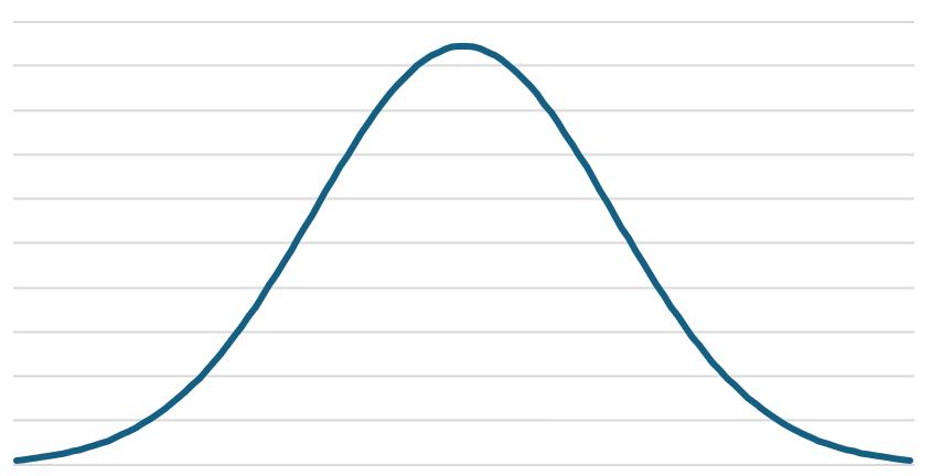
Normal distribution probably needs no introduction, but let’s quickly summarize how it is defined and what are its properties. As shown on Figure 1, normal distribution follows a well-known bell curve centered around the mean . Width of the bell curve is defined by the standard deviation . These are the input parameters that adjust the shape of the distribution – mean translates the center point and standard deviation stretches the curve.

Normal distribution is defined by the probability distribution function (PDF):
where is the value for which we want to calculate the probability The first part of the definition ( is the normalization constant which ensures that this PDF integrates to one. Notice that this formula can be significantly simplified for case when and . This setting deserves a special name – a standard normal distribution.
This PDF has an infinite range, but its interesting property is that 95.4% of samples falls into range and 99.7% falls within . This means that very few samples are generated more than away from the mean value. The probability of sampling numbers past actually falls below . This has a practical implication when working with normally distributed samples – we can focus on the range and be sure that vast majority samples will fall there, e.g., when constructing a kernel for gaussian blur, we can safely take only the samples within around the mean.
A classical approach to sampling any distribution is to use inverse transform sampling. Here, we need to find a cumulative distribution function (CDF) of our distribution, invert it, and use that to transform uniformly distributed random number into our target distribution. For normal distribution, its inverse CDF has a special name – the probit function.
If you want to learn about CDF and its inverse for the normal
distribution, the article “How to generate Gaussian
samples”
goes into great detail. For us, the important thing is that the CDF
contains the error
function , and
inversion requires its inverse . This is the strange
ErfInv() function I stumbled across in the beginning.
For the standard normal distribution, the CDF and its inverse are:
This leads to a straightforward sampling routine we have seen in “Ray Tracing Gems”:
float sampleNormalDistributionInvCDF(float u, float mean, float standardDeviation){ return mean + SQRT_TWO * standardDeviation * erfinv(2.0f * u - 1.0f);}The problem with the inverse error function is that we cannot evaluate it directly. In practice, we need to use one of many available approximations. The quality of samples that we’ll generate depends on the quality of this approximation.
One such approximation was described in “A handy approximation for the error function and its inverse” and its efficient implementation can be found on StackOverflow:
float erfinv(float x){    float tt1, tt2, lnx, sgn;    sgn = (x < 0.0f) ? -1.0f : 1.0f;    x = (1.0f - x) * (1.0f + x);    lnx = log(x);    tt1 = 2.0f / (3.14159265359f * 0.147f) + 0.5f * lnx;    tt2 = 1.0f / (0.147f) * lnx;
    return (sgn * sqrt(-tt1 + sqrt(tt1 * tt1 - tt2)));}
You can plug this directly into the sampling routine and it will start working.
The erfinv() approximation in the above listing is fast, but its error
is up to 0.0035 for inputs approaching one (for inputs near the zero the
error is much smaller). Luckily, there is one more GPU-friendly
approximation that you can use, introduced in “Approximating the erfinv
function”.
It is based on polynomial approximations and much more precise. The
error is only around , but it is also slower. Inversion method
with this erfinv() approximation actually becomes slower than the
method 2 we are going to introduce next. You can use this approximation
if higher accuracy is more important than speed – the impact this has on
the quality of generated samples is discussed in the Evaluation section.
Full listing of this function can be found in the original article, and
in our code on
Github.
This method was described in 1958 by Box and Muller in “A Note on the Generation of Random Normal Deviates”. This is a transformation method that transforms two uniformly distributed random numbers into two numbers distributed according to the normal distribution. These are completely independent, so you can only use one and throw another away in case you don’t need it. The algorithm is quite elegant, its HLSL implementation is:
float2 sampleGaussBoxMuller(float2 u, float mean, float standardDeviation){    const float a = standardDeviation * sqrt(-2.0f * log(1.0f - u.x));    const float b = TWO_PI * u.y;
    return float2(cos(b), sin(b)) * a + mean;}
A requirement stated for this algorithm is that first random number cannot be zero. Wikipedia pseudocode deals with this by generating the first input random number in a loop until it is non-zero. In our code, we go around this by making use of the RNG that generates random number in the interval , which is open on the right side. Therefore, it never generates one, so we take value for the Box-Muller algorithm to avoid the zero. The RNG that we used for our tests was described in the chapter “Reference Path Tracer” in “Ray Tracing Gems 2”.
Box-Muller transform is generally more precise than inverse transform method (it doesn’t suffer from the approximation of the error function), but at the cost of using sine and cosine functions. It also requires two input random numbers instead of one, needing more invocations of the input RNG. This makes it slower, but it also always generates two completely independent random numbers, which can offset this cost in case we have use for both.
Even if we don’t immediately use both numbers, we can cache one for
later use. If you don’t use one of the generated numbers at all, the
compiler will optimize out the unused sine or cosine function call to
make it faster, but still not as fast as the inversion method with
fastest erfinv() approximation.
Sidenote: some architectures provide a combined sincos instruction, which may speed up this method.
While doing research for this blog, I found several articles that produced (the variance) to drive the gaussian distribution instead of the non-squared . I think this creates some confusion whether we should use or as the input to the sampling routine, especially because the PDF definition only contains . All the sampling routines that I tried take non-squared as the input parameter. If you’re in doubt which one is used by the sampling method available to you, you can simply draw a bunch of random numbers and check their histogram to see in which interval falls 95.4% of them – it should be in the interval .
To evaluate the speed of each method, I setup a simple test running a compute shader which generated 2 samples per thread, running in a grid of threads. For this test, only one of Box-Muller results was used. I also ran a second test to generate twice as many samples per thread to evaluate how Box-Muller performs in the setting when both generated samples are used. Results are summarized in Table 1. The GPU used for testing was AMD Radeon RX 7900XT.
| 1 sample | 2 samples | |
|---|---|---|
(Method 1) Inverse transform with fast erfinv() | 0.72ms | 1.43ms |
(Method 1) Inverse transform with precise erfinv() | 0.96ms | 2.15ms |
| (Method 2) Box-Muller transform | 0.84ms | 0.95ms |
Table 1 - Speed evaluation of discussed methods. Highest speed in each column is highlighted in bold.
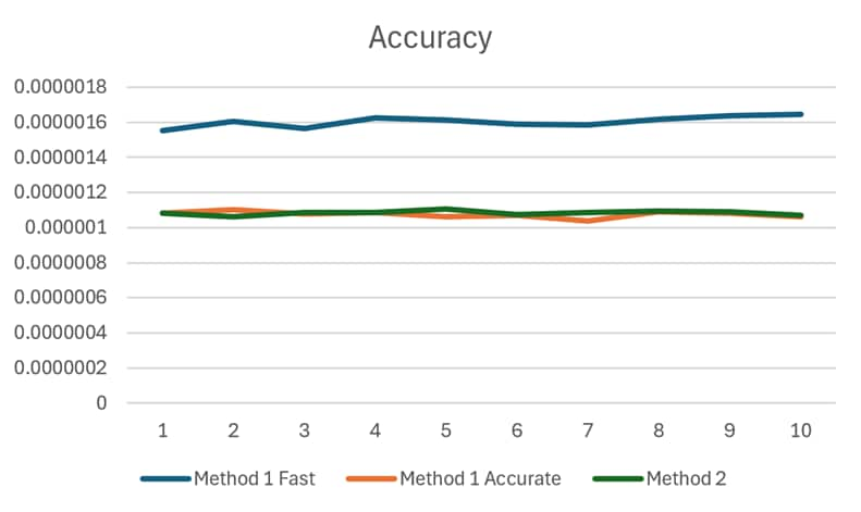
For the evaluation of quality of generated samples, I used a test where
I constructed histograms of samples generated by each method
and compared them to an ideal normal distribution. This was repeated 10
times to make sure this approach provided consistent results. Test was
done for 3 configurations: (1) Method 1 with fast erfinv(), (2) Method
1 with precise erfinv() and (3) Method 2. As shown in Figure 2, method
1 with precise erfinv() has the same accuracy as the method 2. Method
1 with fast erfinv() is worse by about 50%.

For highest speed, I recommend starting with the inverse transform
method combined with a fast approximation for the erfinv() function.
Inverse transform is also preferred method when using low-discrepancy
sequences as it preserves their properties better. It is also faster
than Box-Muller method if we are only interested in drawing a single
random number (assuming we use fast erfinv()). If you don’t care about
the ultimate speed, and want to use inverse transform method (e.g.
because you’re using low-discrepancy sequences), you can increase its
accuracy by using precise erfinv() to the same level of accuracy as
the Box-Muller transform.
If we need two numbers, then Box-Muller becomes faster, as it can generate two numbers in one invocation for the similar cost as it can generate one, and it is more precise.
Another consideration is about the quality of generated samples wrt. the input samples. Some sources state that Box-Muller is more sensitive to quality of the uniform random numbers fed to it, especially with common LCG-based generators, so you need to be careful about your RNG used for initial samples. More about this can be found in “Generating low-discrepancy sequences from the normal distribution: Box–Muller or inverse transform?”.
Before we conclude, I want to quickly mention one more method – the Marsaglia polar method, which is derived directly from the Box-Muller transform. This method got rid of the sine and cosine calculation of Box-Muller making it more numerically stable, robust and possibly faster. The disadvantage is that it is a form of rejection sampling and requires a while loop at the beginning to generate two random numbers distributed within a unit circle. Therefore, it is not very suitable for GPU applications as the execution path becomes unpredictable. My tests shown that because of this, it is also considerably slower than other methods described here. For these reasons, I am only mentioning this method here without going into details.
We have explored two methods for sampling a normal distribution suitable for GPUs. Code for both methods without dependencies is publicly available on Github. If you want to learn about more algorithms for sampling this distribution, I recommend the study titled Gaussian Random Number Generators. I want to thank Carsten Benthin for helpful comments on this article.
Links to third party sites are provided for convenience and unless explicitly stated, AMD is not responsible for the contents of such linked sites and no endorsement is implied.
