Understanding concurrency (and what breaks it) is extremely important when optimizing for modern GPUs. Modern APIs like DirectX® 12 or Vulkan® provide the ability to schedule tasks asynchronously, which can enable higher GPU utilization with relatively little effort.

Why concurrency is important

Rendering is an embarrassingly parallel task. All triangles in a mesh can get transformed in parallel and non-overlapping triangles can get rasterized in parallel. Consequentially GPUs are designed to do a lot of work in parallel. E.g. Radeon™ Fury X GPU consists of 64 Compute Units (CUs), each of those containing 4 Single-Instruction-Multiple-Data units (SIMD) and each SIMD executes blocks of 64 threads, which we call a “wavefront”. Since latency for memory access can cause significant stalls in shader execution, up to 10 wavefronts can be scheduled on each SIMD simultaneously to hide this latency.

There are several reasons why the actual number of wavefronts in flight is often lower than this theoretical maximum. The most common reasons for this are:

• A Shader uses many Vector General Purpose Registers (VGPR): E.g. if a shader uses more than 128 VGPR only one wavefront can get scheduled per SIMD (for details on why, and how to compute how many wavefronts a shader can run, please see the article on how to use CodeXL to optimize GPR usage).
• LDS requirements: if a shader uses 32KiB of LDS and 64 threads per thread group, this means only 2 wavefronts can be scheduled simultaneously per CU.
• If a compute shader doesn’t spawn enough wavefronts, or if lots of low geometry draw calls only cover very few pixels on screen, there may not be enough work scheduled to create enough wavefronts to saturate all CUs.
• Every frame contains sync points and barriers to ensure correct rendering, which cause the GPU to become idle.

Asynchronous compute can be used to tap into those GPU resources that would otherwise be left on the table.

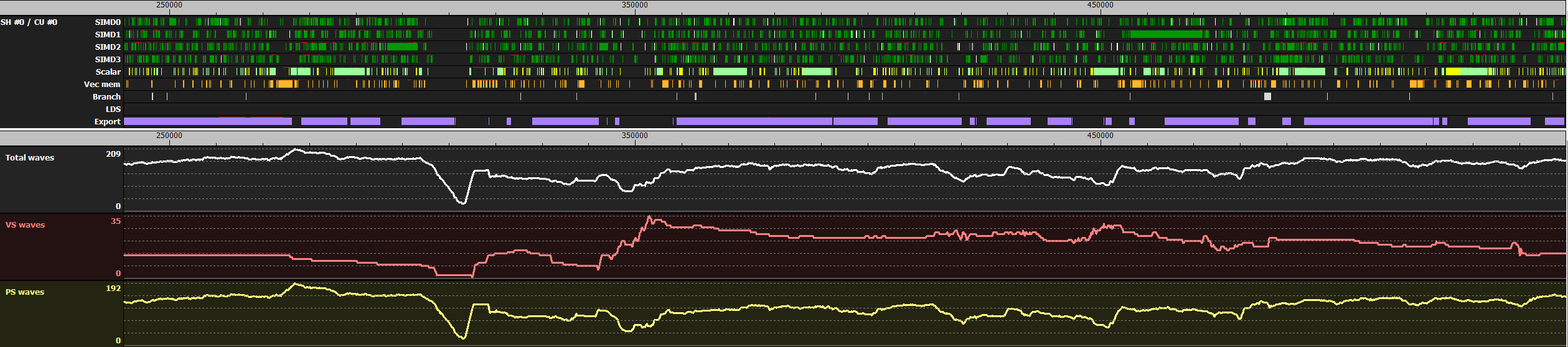
The two images below are screenshots vizualizing what is happening on one shader engine of a Radeon™ RX480 GPU in typical parts of a frame. The graphs are generated by a tool we use internally at AMD to identify optimization potential in games.
The upper sections of the images show the utilization of the different parts of one CU. The lower sections show how many wavefronts of different shader types are launched.

The first image shows ~0.25ms of G-Buffer rendering. In the upper part the GPU looks pretty busy, especially the export unit. However it is important to note that none of the components within the CU are completely saturated.

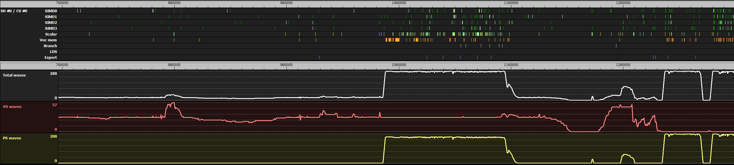
The second image shows 0.5ms of depth-only rendering. In the left half no PS is used, which results in very low CU utilization. Near the middle some PS waves get spawned, probably due to rendering transparent geometry via alpha testing (but the reason is not visible in those graphs). In the rightmost quarter there are a few sections where the total number of waves spawned drops to 0. This could be due to render targets getting used as textures in the following draw calls, so the GPU has to wait for previous tasks to finish.

Improved performance through higher GPU utilization

As can be seen in those images, there is a lot of spare GPU resources in a typical frame. The new APIs are designed to provide developers with more control over how tasks are scheduled on the GPU. One difference is that almost all calls are implicitly assumed to be independent and it’s up to the developer to specify barriers to ensure correctness, such as when a draw operation depends on the result of a previous one. By shuffling workloads to improve batching of barriers, applications can improve GPU utilization and reduce the GPU idle time spent in barriers each frame.

An additional way to improve GPU utilization is asynchronous compute: instead of running a compute shader sequentially with other workloads at some point in the frame, asynchronous compute allows execution simultaneously with other work. This can fill in some of the gaps visible in the graphs above and provide additional performance.

To allow developers to specify which workloads can be executed in parallel, the new APIs allow applications to define multiple queues to schedule a task onto.
There are 3 types of queues:

• Copy Queue(DirectX® 12) / Transfer Queue (Vulkan®): DMA transfers of data over the PCIe bus
• Compute queue (DirectX® 12 and Vulkan®): execute compute shaders or copy data, preferably within local memory
• Direct Queue (DirectX® 12) / Graphics Queue (Vulkan®):  this queue can do anything, so it is similar to the main device in legacy APIs

The application can create multiple queues for simultaneous use: in DirectX® 12 an arbitrary number of queues for each type can be created, while in Vulkan® the driver will enumerate the number of queues supported.
GCN hardware contains a single geometry frontend, so no additional performance will be gained by creating multiple direct queues in DirectX® 12. Any command lists scheduled to a direct queue will get serialized onto the same hardware queue. While GCN hardware supports multiple compute engines we haven’t seen significant performance benefits from using more than one compute queue in applications profiled so far. It is generally good practice not to create more queues than what the hardware supports in order to have more direct control on command list execution.

Build a task graph based engine

How to decide which work to schedule asynchronously? A frame should be considered a graph of tasks, where each task has some dependencies on other tasks. For example, multiple shadow maps can be generated independently, and this may include a processing phase with a compute shader generating Variance Shadow Map (VSM) using shadow map inputs. A tiled lighting shader, processing all shadowed light sources simultaneously, can only start after all shadow maps and the G-Buffer have finished processing. In this case VSM generation could run while other shadow maps get rendered, or batched during G-Buffer rendering.
Similarly generating ambient occlusion depends on the depth buffer, but is independent of shadows or tiled lighting, so it’s usually a good candidate for running on the asynchronous compute queue.

In our experience of helping game developers come up with optimal scenarios to take advantage of asynchronous compute we found that manually specifying the tasks to run in parallel is more efficient than trying to automate this process. Since only compute tasks get scheduled asynchronously, we recommend to implement a compute path for as many render workloads as possible in order to have more freedom in determining which tasks to overlap in execution.
Finally, when moving work to the compute queue, the application should make sure each command list is big enough. This will allow performance gains from asynchronous compute to make up for the cost of splitting the command list and stalling on fences, which are required operations for synchronizing tasks on different queues.

How to check if queues are working as expected

I recommend using GPUView to ensure asynchronous queues in an application are working as expected. GPUView will visualize which queues are used, how much work each queue contains and, most importantly, if the workloads are actually executed in parallel to each other.

Under Windows® 10 most applications will at least show one 3D graphics queue and a copy queue, which is used by Windows for paging. In the following image you can see one frame of an application using an additional copy queue for uploading data to the GPU. The grab is from a game in development using a copy queue to stream data and upload dynamic constant buffers before the frame starts rendering. In this build of the game the graphics queue needed to wait for the copy to finish, before it could start rendering. In the grab it can also be seen, that the copy queue waits for the previous frame to finish rendering before the copy starts:

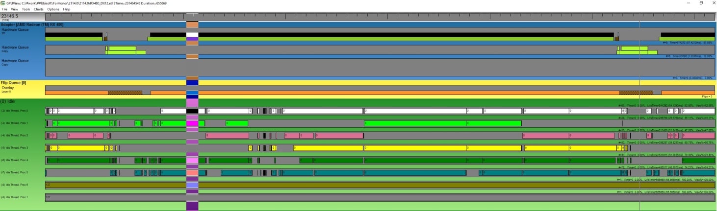
In this case, using the copy queue did not result in any performance advantage, since no double buffering on the uploaded data was implemented. After the data got double-buffered, the upload now happens while the previous frame is still being processed by the 3D queue and the gap in the 3D queue is eliminated. This change saved almost 10% of the total frame time.

The second example shows two frames of the benchmark scene in Ashes of the Singularity, a game, which makes heavy use of the compute queue:

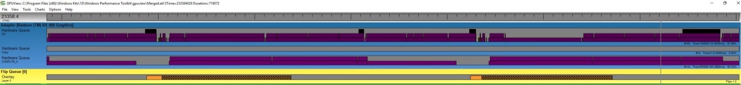
The asynchronous compute queue is used for most of the frame. It can be seen from the trace that the graphics queue is not stalled while waiting on the compute queue, which is a good starting point to ensure asynchronous compute is best placed to provide performance gains.

What could possibly go wrong?

When using asynchronous compute it needs to be taken into account that even though the command lists on different queues are executed in parallel, they still share the same GPU resources.

• If resources are located in system memory accessing those from Graphics or Compute queues will have an impact on DMA queue performance and vice versa.
• Graphics and Compute queues accessing local memory (e.g. fetching texture data, writing to UAVs or performing rasterization-heavy tasks) can affect each other due to bandwidth limitations
• Threads sharing the same CU will share GPRs and LDS, so tasks that use all available resources may prevent asynchronous workloads to execute on the same CU
• Different queues share their caches. If multiple queues utilize the same caches this can result in more cache thrashing and reduce performance

Due to the reasons above it is recommended to determine bottlenecks for each pass and place passes with complementary bottlenecks next to each other:

• Compute shaders which make heavy use of LDS and ALU are usually good candidates for the asynchronous compute queue
• Depth only rendering passes are usually good candidates to have some compute tasks run next to it
• A common solution for efficient asynchronous compute usage can be to overlap the post processing of frame N with shadow map rendering of frame N+1
• Porting as much of the frame to compute will result in more flexibility when experimenting which tasks can be scheduled next to each other
• Splitting tasks into sub-tasks and interleaving them can reduce barriers and create opportunities for efficient async compute usage (e.g. instead of “for each light clear shadow map, render shadow, compute VSM” do “clear all shadow maps, render all shadow maps, compute VSM for all shadow maps”)

It is important to note that asynchronous compute can reduce performance when not used optimally. To avoid this case it is recommended to make sure asynchronous compute usage can easily be enabled or disabled for each task. This will allow you to measure any performance benefit and ensure your application runs optimally on a wide range of hardware.