
D3D12 Memory Allocator
The D3D12 Memory Allocator (D3D12MA) is a C++ library that provides a simple and easy-to-integrate API to help you allocate memory for DirectX®12 buffers and textures.
In computer graphics, we rarely encounter continuous data. We often work with digital data, and in the context of geometric modeling, this means we typically work with polygon meshes rather than procedural surfaces like Bézier patches. The most popular technique for constructing digital three-dimensional objects in dedicated modeling software is polygon modeling. The result of the creation phase is a set of polygons (mesh), where the polygons in the mesh can share vertices and edges with other polygons.
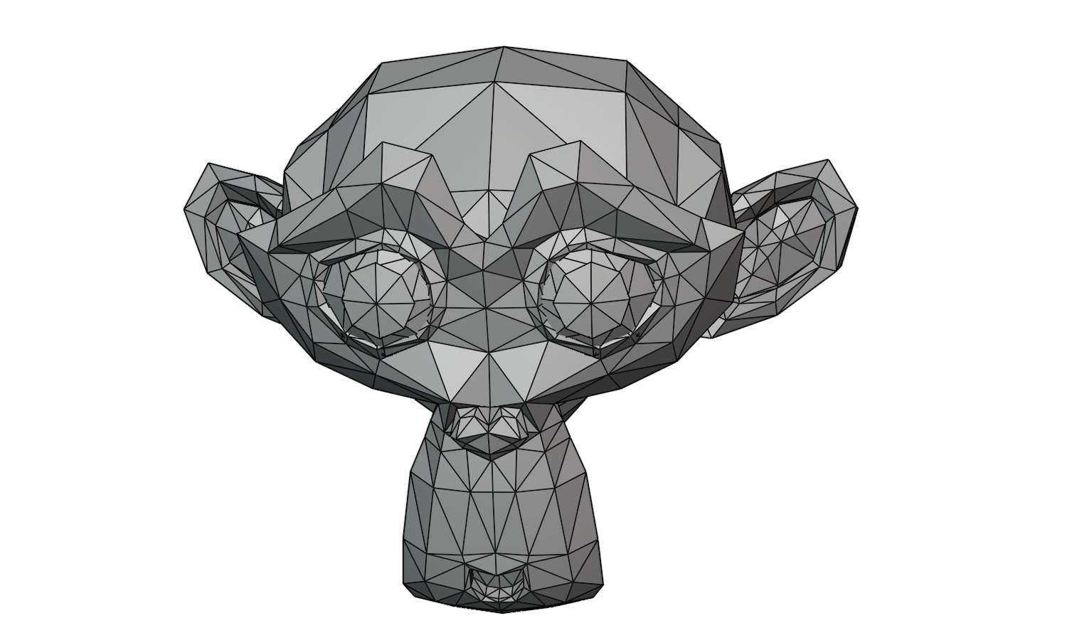
Although users can create various types of surfaces (e.g., non-manifold), the most common surface is the topological 2-manifold. In short, a 2-manifold is a mathematical concept in topology, where the space locally resembles the Euclidean plane in . Essentially, every point on a 2-manifold has a neighborhood that looks like a piece of the plane.
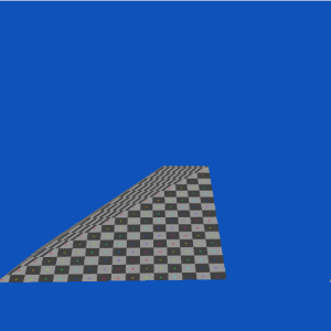
| Examples of 2-manifold mesh triangle-based | Examples of 2-manifold mesh quad-based |
|
|
At the vertices of a polygon, users can store additional data (per-vertex attributes), such as vertex normals (for simulating curved surfaces), texture coordinates (for texture mapping), or RGBA color.
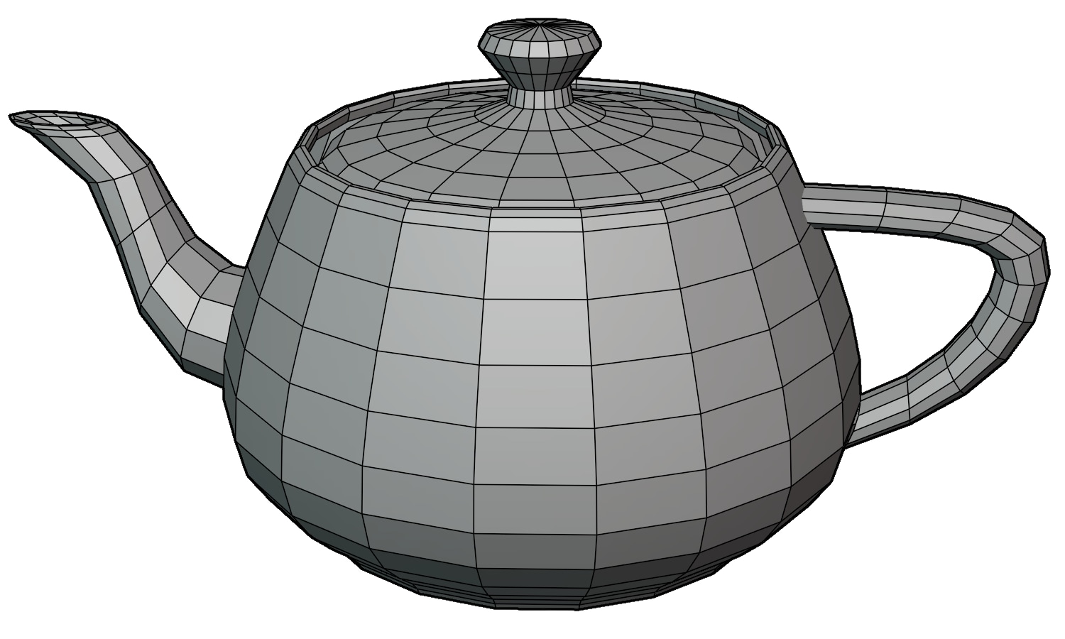
In theory, all types of polygons can be used. In practice, however, 3D graphics artists most commonly use triangles and quadrilaterals. These polygons are typically referred to as topology primitives in computer graphics APIs (such as Microsoft DirectX® or Vulkan®). From an artist’s point of view, quadrilaterals are more advantageous because they are easier to work with. The properties of modeling based on quadrilaterals include:
The ease of generating grid-like surfaces.
Creating a topology that provides an edge flow that can be easily adjusted (when adding or deleting edge loops).
Producing a predictable result for subdivision algorithms.
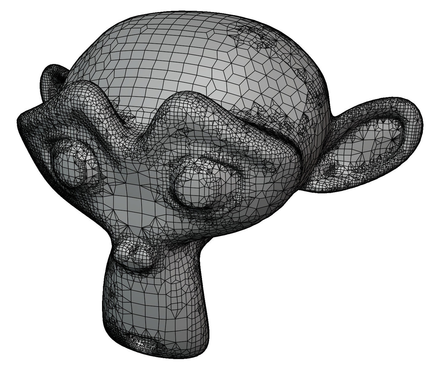
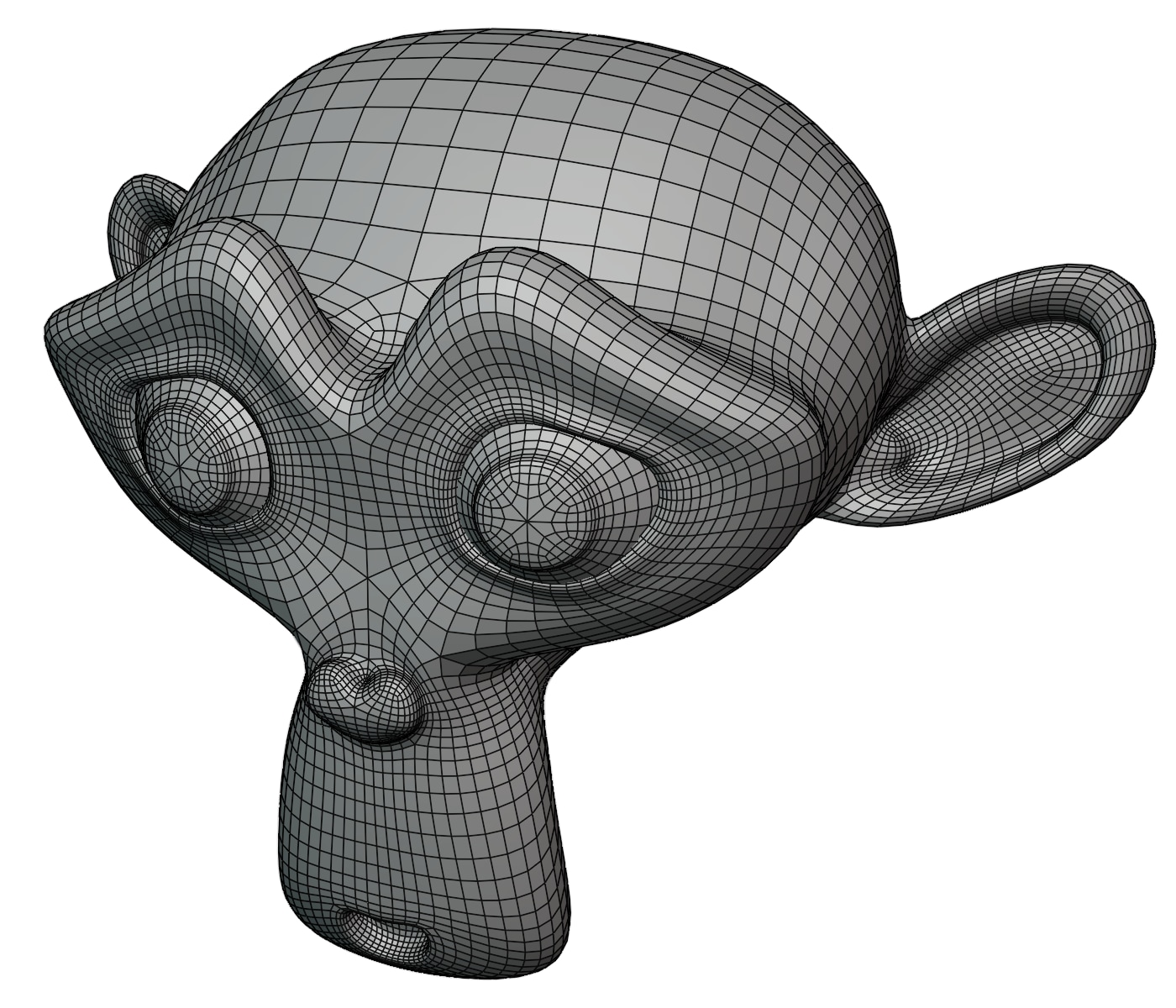
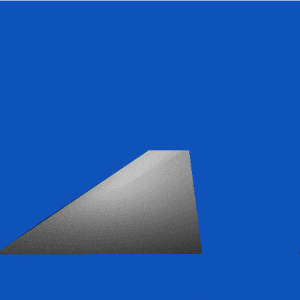
| not clean looking mesh | clean looking mesh |
|
|
These arguments make the quadrilateral-based topology preferred by artists when modeling 3D objects.
Long ago, GPUs abandoned support for hardware accelerated quadrilaterals (or polygons consisting of more than 4 vertices) rasterization, therefore also interpolation of vertex attributes contained in their vertices (line rendering is for a different story). The only polygon that has hardware accelerated implementation of rasterization and interpolation of parameters is the triangle. There are very good reasons why it was the triangle that won the race I just name a few:
Triangulation Theorem: This theorem states that a mesh of triangles can approximate even complex surfaces.
Triangle vertices always lie on the same plane: This is due to the fact that any three non-collinear points will always define a plane in three-dimensional space.
Barycentric Coordinates: This coordinate system is used in geometry to express the position of a point within a triangle. These coordinates can be used for interpolation of vertex attributes across the surface of a triangle.
Less complexity of the circuit: Supporting rasterization and interpolation for triangles only requires fewer transistors, which means this functionality occupies less space on the chip. This can result in a smaller (and cheaper to produce) chip, or the saved space can be used for other functionalities.
Triangles are the foundation of real-time computer graphics, as reflected in the primitive topology supported by graphics APIs. All other polygon types used in meshes must be converted into triangles. When a modeling application allows quad-mesh construction, the visualization of this mesh is not based on quadrilaterals. Instead, the application converts them into triangle meshes. This necessary conversion can introduce discontinuities in interpolated vertex attributes (such as texture coordinates, vertex normal vectors, and vertex colors) on the quadrilateral surface.
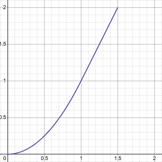
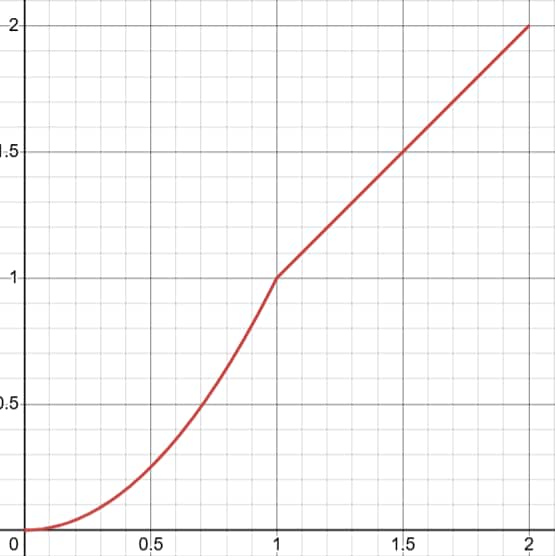
In the case of the topic covered in this article, the discontinuity of refers to the point at which the piecewise function is continuous, but its first derivative is not. In other words, the piecewise function itself has no jumps or breaks, but the slope (or rate of change) of the piecewise function has jumps or breaks.
| continuity | discontinuity | |
| piecewise function |
|
|
| first derivative |
|
|
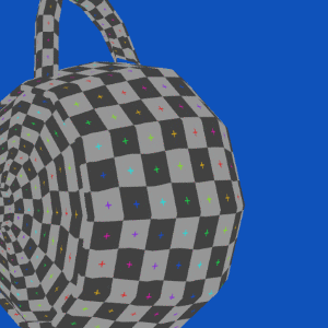
For rasterization of quadrilaterals as two triangles, discontinuity in the interpolation of vertex attributes is most visible along the newly created edge that splits the quadrilateral into two triangles.
| Vertex Color | Texture Coordinates | Vertex Normal |
 |  |  |
 |  |  |
 |  |  |
The purpose of this article is to propose a new method that preserves continuity over the common edge of two generated triangles from convex quadrilaterals. This new method is based on an algebraic solution for the Bilinear interpolation coefficient expressed in Barycentric coordinates. Bilinear interpolation has the advantage of being the simplest interpolation from an algebraic perspective. Consequently, the computational overhead is negligibly small. Additionally, linear interpolation allows for the easy construction of other types of interpolation, such as polynomial interpolation. The algebraic solution will then be implemented and tested using the three available hardware-accelerated pipelines supported by GPU hardware.
Currently, efforts to address the problem outlined in this article can be categorized into the following approaches:
The first approach is not to eliminate the issue but to minimize it. This is achieved by subdividing the quadrilateral until rendering artifacts become imperceptible to the observer or are less noticeable than the aliasing artifacts created during rasterization.
Quadrilateral subdivision can be performed dynamically (at application runtime) using a hardware-accelerated Tessellation Shaders stage.
| Tessellation level 1 | Tessellation level 2 | Tessellation level 3 | Tessellation level 4 | Tessellation level 5 |
 |  |  |  |  |
Alternatively, quadrilateral subdivision can be performed statically (during the content creation phase) using dedicated tools provided by modeling software, such as the Blender® Subdivision Surface Modifier.
| Mesh in Blender before usage of Subdivision Surface Modifier | Mesh in Blender after usage of Subdivision Surface Modifier |
|
|
Subdividing meshes (at application runtime or not) effectively reduces the visibility of all types of discontinuities to the observer, but at the expense of decreasing performance and/or increasing memory overhead in the mesh rendering process.
A different attempt to solve the problem was offered in the article A quadrilateral rendering primitive, where the authors proposed hardware-accelerated quadrilateral rasterization. For vertex attribute interpolation inside quadrilaterals (which may be non-planar), the authors chose to use mean value coordinates. However, these coordinates yield results similar to those of bilinear interpolation. The following caveats can be pointed out:
In the calculation of mean value coordinates, transcendental functions are used. The values of these functions can be determined with predetermined precision. However, from a performance perspective, they introduce a certain overhead, depending on the hardware implementation of the calculation of transcendental functions.
Mean value coordinates interpolation does not generate straight lines, which might not be desirable for users. This hardware solution has not yet been implemented using the GPU (at the time of writing this article). However, the authors of Barycentric quad rasterization attempted to implement it using the Geometry Shader pipeline available in modern GPUs. The presented implementation has a disadvantage: it uses double-precision floating-point variables, which significantly impact performance overhead. GPUs for real-time rendering are primarily designed to support single-precision floating-point calculations.
Other authors, such as Inigo Quilez inverse bilinear interpolation – 2010 and Nathan Reed Quadrilateral Interpolation, Part 2, have observed the advantages of bilinear interpolation and proposed solutions through implementations using the Fragment Shader.
The presented solutions demonstrate the implementation of bilinear interpolation for quadrilaterals, but they only show how to do it for a single quadrilateral and for its texture coordinate vertex attribute. They do not address how to apply it in real-life three-dimensional mesh models.
The method presented in the article consists of an equation that can express Bilinear interpolation coefficients using Barycentric coordinates of one of the two triangles into which each convex quadrilateral can be divided.
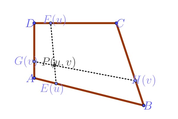
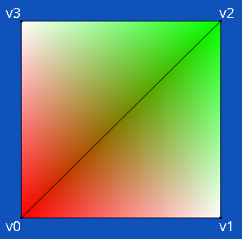
The Euclidean coordinates of every point in a given quadrilateral on the plane can be expressed as a Bilinear interpolation of the Euclidean coordinates of its vertices.
The line segment is parameterized as ,
the line segment is parameterized as ,
the line segment is parameterized as ,
the line segment is parameterized as .
The point is the intersection of the two segments and .
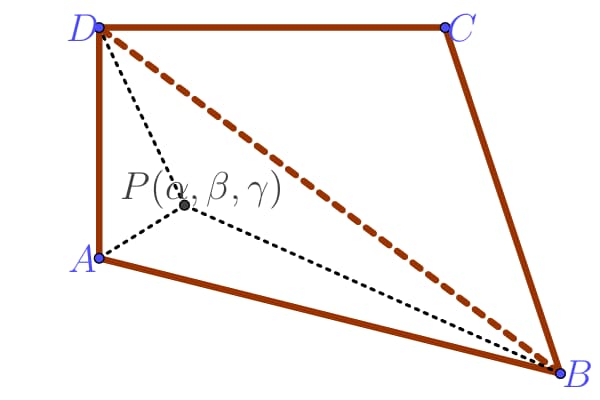
Alternatively, the Euclidean coordinates of point can be expressed as a Barycentric coordinates of
a triangle ABD \
where are positive real numbers such that ..
This can be shown geometrically in two-dimensional space.
| Bilinear interpolation inside quadrilateral | Barycentric interpolation inside triangle |
|
|
The Euclidean coordinates of point are the same whether it is inside the quadrilateral or the triangle .
Depending on the Euclidean coordinates of point , it may lie inside triangle or triangle . There is a system of equations that describe the coordinates of point using the vertices of quadrilateral and the Bilinear interpolation coefficients , as well as the vertices of triangles or and the Barycentric coordinates for the same point .
The coordinates of point in can be calculated using Barycentric coordinates and Bilinear interpolation coefficients and , which can be expressed by the following two independent set of equations:
The coordinates of point in can be calculated using Barycentric coordinates and Bilinear interpolation coefficients and , which can be expressed by the following two independent sets of equations:
The equations can be reduced to the form:
We can further simplify using:
to a two-system of equations:
Now, solving the two systems of equations for and leads to the problem of solving two quadratic equations:
Embedding this solution in at the plane with the surface normal vector for a triangle , the equation can be written as:
where is the cross product in and is the dot product in .
Substituting the triple dot product into the equation:
the final two equations are as follows:
The last step is to solve these two quadratic equations for the parameters and .
The equation can be used to calculate bilinear interpolation coefficients and for any quadrilateral in three-dimensional space. This is because if a quadrilateral is embedded in any plane in , it can be transformed isometrically to the plane , and the premise still holds after isometric mapping.
It is worth noting that the above equations show that the bilinear interpolation coefficients and depend on all four Euclidean coordinates of the vertices in the quadrilateral. If we are dealing with static meshes, these coefficients can be calculated in advance (this is not necessary at runtime). However, if we are working with dynamic (animated) meshes, it is necessary to calculate these coefficients at runtime. Therefore, we need to use a Graphics Pipeline stage where we still have access to all four positions of the vertices of the quadrilateral.
When rendering quadrilaterals limited to parallelograms, the solution is much simpler because . This fact can be deduced after a quick analysis.
Vector is described as . In parallelograms, the vector from the first parenthesis , by definition, has the same length as the vector but in the opposite direction. Thus, the sum of these vectors is always the zero vector.
Therefore, when , we are no longer dealing with a quadratic equation, but with a linear equation, making the solution much simpler:
This simpler case has already been described, and the solution can be found in How to Correctly Interpolate Vertex Attributes on a Parallelogram Using Modern GPUs?.
The hardware-accelerated implementation of the algebraic solution presented in the previous section can be achieved using three different Graphics Pipeline stages: Geometry Shader, Tessellation Shader, and Mesh Shader. This three-way implementation demonstrates that the technique is feasible on GPU hardware released as far back as 2008. The following source code uses the GLSL shading language.
The table below describes what API versions and extensions are necessary to implement the presented technique:
| Vulkan® | DirectX® | OpenGL® | |
| Geometry Shader | Vulkan® geometry Shader feature enabled | DirectX® 10 | OpenGL® 3.2 |
| Tessellation Shader | Vulkan® tessellation Shader feature enabled | DirectX® 11 | OpenGL® 4 |
| Mesh Shader | Vulkan® VK_EXT_mesh_shader extension enabled | DirectX® 12 Ultimate | OpenGL® 4 GL_NV_mesh_shader extension enabled |
The implementation of the presented method requires Barycentric coordinates of the currently processed fragment in the Fragment Shader. This is possible when the following extensions are available:
Vulkan® VK_KHR_fragment_shader_barycentric extension.
DirectX® 12 Shader Model 6.1.
OpenGL® 4 GL_NV_fragment_shader_barycentric or GL_AMD_shader_explicit_vertex_parameter.
If the GPU does not support the above extension, there is a way to generate them in the Geometry, Tessellation, or Mesh Shader stage.
The implementation of the new method presented in this article can be divided into the following steps:
Delivering Quadrilateral Primitives to the Graphics Pipeline.
Quadrilateral primitives are not available in modern graphics APIs (excluding the legacy OpenGL GL_QUADS and GL_QUAD_STRIP primitive types). To support quadrilateral-like primitives, use the following methods:
Geometry Shader: With the Geometry Shader stage, adjacency primitives can be used to mimic quadrilateral primitives:
OpenGL® GL_LINES_ADJACENCY
Vulkan® VK_PRIMITIVE_TOPOLOGY_LINE_LIST_WITH_ADJACENCY
DirectX® 12/11 D3D_PRIMITIVE_TOPOLOGY_LINELIST_ADJ
With Tessellation stages, a new Patch primitive was introduced. In this topology, the number of vertices defined in the meshes is not fixed, but the so-called Control Points range from 1 to 32 per Patch. These Control Points can be treated as Control Points of Bézier patches, but they can also be treated as vertices of a polygon. The implementation of the solution presented in this article uses a Patch with 4 Control Points and treats them as vertices of a quadrilateral.
Mesh Shader: Using Mesh Shaders, there are many ways to introduce a quadrilateral primitive into the Graphics Pipeline. This stage was developed to provide more flexibility to the user. Therefore, it is up to the user to generate meshlets that will contain quadrilaterals in some way (this is not within the scope of this article).
The next step is to calculate the constants (using one of the steps above), which will then be used in the Fragment Shader. We need to calculate these constants in one of the above pipeline stages because, in the Fragment Shader, we do not have access to the four attributes of the quadrilateral vertices (the Barycentric coordinate extension, if present, only gives us access to the three attributes of the triangle vertices). By analyzing the algebraic solution of the presented method, we can see that these constants depend on the positions of the vertices of the quadrilateral.
The following function needs to be executed in the Geometry Shader, Tessellation Evaluation Shader, or Mesh Shader.
vec3 calculateConstants(vec3 v0, vec3 v1, vec3 v2, vec3 v3) { const vec3 v10 = v1 - v0; const vec3 v30 = v3 - v0; const vec3 crossv10v30 = cross(v10, v30); const vec3 n = normalize(crossv10v30); const vec3 d = v0 - v1 + v2 - v3; float A_u = dot(n, cross(d, v30)); float A_v = dot(n, cross(d, v10)); const float B = dot(n, crossv10v30); A_u = abs(A_u) < 0.00001 ? 0.0 : A_u; A_v = abs(A_v) < 0.00001 ? 0.0 : A_v; return vec3(A_u, A_v, B); }Where v0, v1, v2, v3 are the Euclidean coordinates of the quadrilateral vertices in the following order:
The calculated values of A_u, A_v and B are then passed to the Fragment Shader.
For Bilinear interpolation to work in a Fragment Shader, we need to be able to fetch all four vertex attributes (such as texture coordinates, vertex normal, and vertex color) in it.
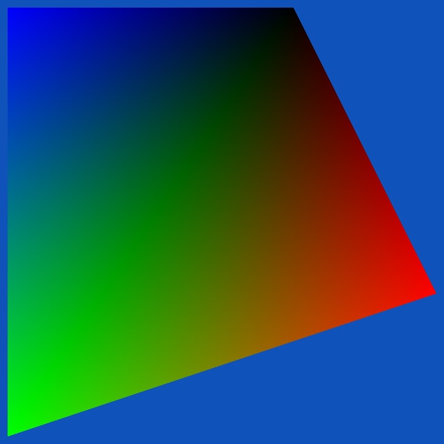
layout (location = 0) pervertexEXT in block{ vec3 Normal; flat vec3 NormalExtra; vec2 Texcoord; flat vec2 TexcoordExtra; vec4 Color; flat vec4 ColorExtra; flat vec3 BaryConstants;} In[];layout(location = 0) in block{ flat vec3 Normal[4]; flat vec2 Texcoord[4]; flat vec4 Color[4]; flat vec3 BaryConstants; vec3 BarycentricCoordinate;} In;When using Barycentric coordinates for interpolation of vertex attributes, the order in which they are defined in the triangle doesn’t matter. However, in the implementation method described in this article, the specific order is important. This order can be visually represented as follows:
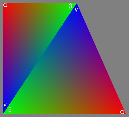
Where red color represents the influence of the Barycentric coordinate, green represents , and blue represents .
This order of Barycentric coordinates can be supplied by hardware when the proper extension is available, or these data can be generated in the Tessellation or Geometry Shader stage.
In the Fragment Shader, the calculation of Bilinear interpolation coefficients and can be done by calling the following function.
vec2 calculateBilinear(float beta, float gamma, float A_u, float A_v, float B) { const float B_u = B; const float B_v = -B; const float B2 = beta * A_v + gamma * A_u; const float t_u = B_u - B2; const float t_v = B_v - B2; const float b_u = t_u / A_u * 0.5; const float b_v = t_v / A_v * 0.5; const float c_u = gamma * B_v; const float c_v = beta * B_u; const float d_u = b_u * b_u - c_u / A_u; const float d_v = b_v * b_v - c_v / A_v; const float s_u = A_u >= 0.0 ? -1.0 : 1.0; const float s_v = A_v >= 0.0 ? 1.0 : -1.0; const float u = A_u != 0.0 ? (-b_u - s_u * sqrt(d_u)) : (-c_u / t_u); const float v = A_v != 0.0 ? (-b_v - s_v * sqrt(d_v)) : (-c_v / t_v); return vec2(u, v); }Where beta is Barycentric coordinate, gamma is Barycentric coordinate, A_u, A_v, B are constants calculated in previous Graphics Pipeline Stage.
When Bilinear interpolation coefficients and are calculated, the interpolation of vertex attributes can be achieved using functions.
vec4 interpolateBilinear(vec4 v0, vec4 v1, vec4 v2, vec4 v3, vec2 uv){ return mix(mix(v0, v1, uv.y), mix(v2, v3, uv.y), uv.x);}vec3 interpolateBilinear(vec3 v0, vec3 v1, vec3 v2, vec3 v3, vec2 uv){ return mix(mix(v0, v1, uv.y), mix(v2, v3, uv.y), uv.x);}vec2 interpolateBilinear(vec2 v0, vec2 v1, vec2 v2, vec2 v3, vec2 uv){ return mix(mix(v0, v1, uv.y), mix(v2, v3, uv.y), uv.x);}float interpolateBilinear(float v0, float v1, float v2, float v3, vec2 uv){ return mix(mix(v0, v1, uv.y), mix(v2, v3, uv.y), uv.x);}Where v0, v1, v2, v3 are the quadrilateral vertex attributes.
For quadrilaterals, which are restricted to parallelograms, implementing the technique described in this article is even simpler.
vec4 calculateConstants(vec4 A, vec4 B, vec4 C, vec4 D){ return A - B + C - D;}vec3 calculateConstants(vec3 A, vec3 B, vec3 C, vec3 D){ return A - B + C - D;}vec2 calculateConstants(vec2 A, vec2 B, vec2 C, vec2 D){ return A - B + C - D;}float calculateConstants(float A, float B, float C, float D){ return A - B + C - D;}Where A, B, C, D are vertex attributes arranged as specified.
The calculated value for each vertex attribute needs to be passed to the Fragment Shader.
vec4 interpolateBilinear(vec4 attribute, vec2 barycentric, vec4 extraVal){ return attribute + barycentric.x * barycentric.y * extraVal;}vec3 interpolateBilinear(vec3 attribute, vec2 barycentric, vec3 extraVal){ return attribute + barycentric.x * barycentric.y * extraVal;}vec2 interpolateBilinear(vec2 attribute, vec2 barycentric, vec2 extraVal){ return attribute + barycentric.x * barycentric.y * extraVal;}float interpolateBilinear(float attribute, vec2 barycentric, float extraVal){ return attribute + barycentric.x * barycentric.y * extraVal;}Where attribute represents a value interpolated by traditional Barycentric interpolation (available in the Fragment Shader), barycentric is a vec2 data type containing the fragments’ and Barycentric coordinates, and extra is a constant calculated in the previous Geometry, Tessellation, Mesh Shader stage.
The output of the algebraic solution presented in this article remains consistent across different implementations. Depending on the type of vertex attributes, the results can be summarized in the following table.
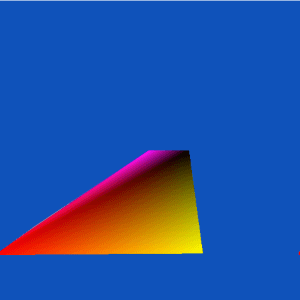
| Vertex Attribute | Barycentric interpolation | Bilinear interpolation using the solution presented in the article |
| Color | | 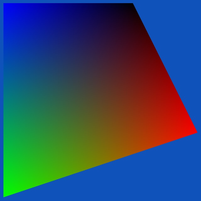 |
| Texture coordinate | | 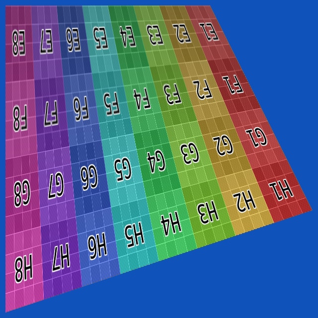 |
| Normal | |  |
| Color | |  |
| Texture coordinate | |  |
| Normal | |  |
| Color | | 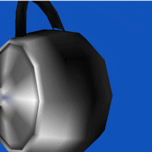 |
| Texture coordinate | | 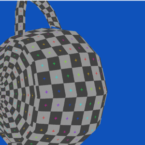 |
| Normal | | 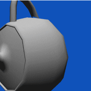 |
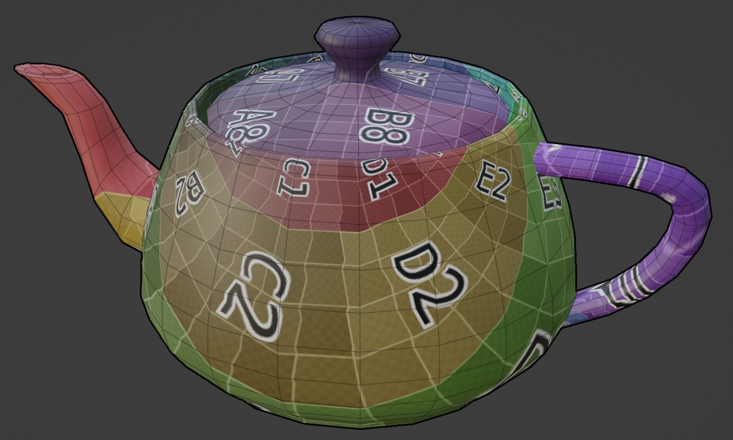
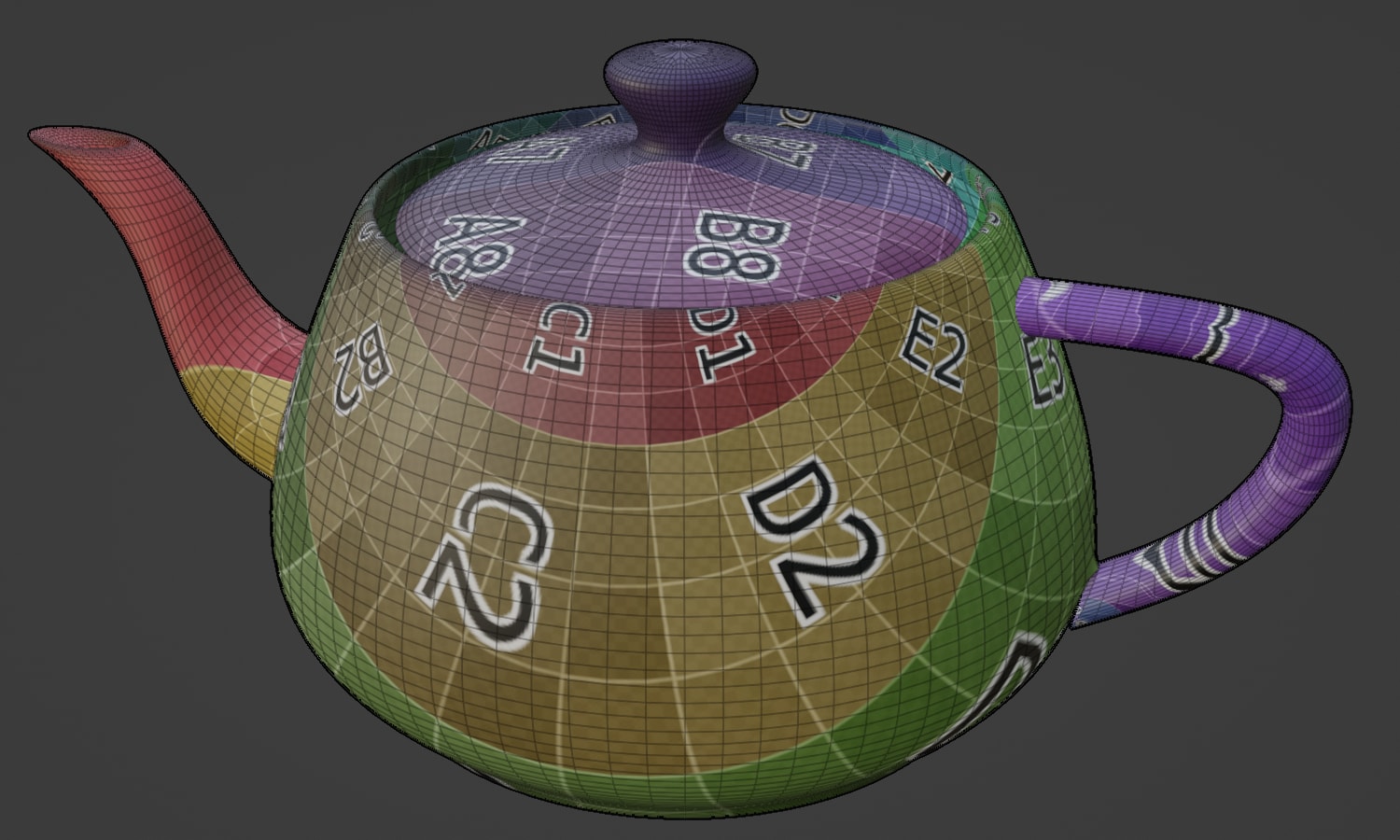
| Mesh Example | 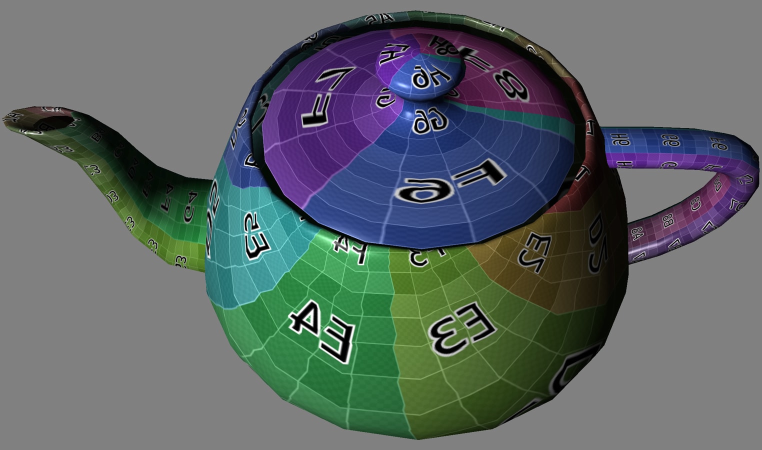 |  |
| Animation Example | 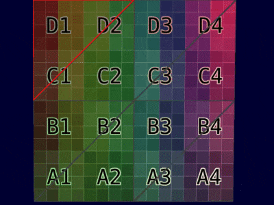 | 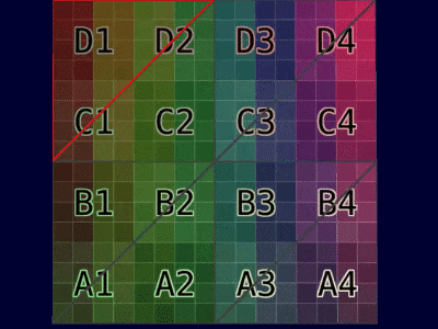 |
As presented in this article, the algebraic solution for Bilinear interpolation using Barycentric coordinates can be implemented through APIs such as Vulkan® or DirectX®. This implementation leverages hardware-accelerated rendering on GPUs. The paper proposes three different implementations based on the available Graphics Pipeline supported by the GPU. These implementations enable the use of the new method on GPUs (both PCs and mobile devices) ranging from models released in 2008 to the latest versions.
Blender is a registered trademark of the Blender Foundation in EU and USA. DirectX is a registered trademark of Microsoft Corporation in the US and other jurisdictions. OpenGL® and the oval logo are trademarks or registered trademarks of Hewlett Packard Enterprise in the United States and/or other countries worldwide. Vulkan and the Vulkan logo are registered trademarks of the Khronos Group Inc.