Profiling video memory with Windows® Performance Analyzer

Budgeting, measuring and debugging video memory usage is essential for the successful release of game titles on Windows. As a developer, this can be efficiently achieved with the help of Microsoft®’s Windows® Performance Analyzer (WPA) tool and with a general understanding of how video resources are managed by the operating system.

Installing WPA

Windows Performance Analyzer is part of the Windows Performance Toolkit, which is part of the Windows 10 SDK. When installing the Windows 10 SDK, make sure the Windows Performance Toolkit box is checked. The typical file path for the install is C_:\Program Files (x86)\Windows Kits\10\Windows Performance Toolkit\_. In that folder there is a perfcore.ini file that will need to be edited to enable video the GPU segment usage tab, which is the one needed for video memory profiling. Perfcore.ini contains a list of .dll files and perf_dx.dll needs to be added to the list.

Capturing an .etl profile

By default, a log.cmd script for triggering capturing is included with the installation. When started, activity is captured for the entire machine, so all processes are included. Administrator privileges are required when running this script. To exemplify, typical steps are:

1. Open a command prompt with administrator privileges. One easy way to do is to type cmd in the Windows Search Box and when the Command Prompt menu options appears, right click on it and select Run as administrator.
2. Run the target app with the settings of interest and set up/prepare a test case.
3. If the machine does not have multiple display monitors and the app is running fullscreen, Alt-Tab can be used to switch to the command prompt and back. Run cmd from the command prompt by entering its path, which would likely be C_:\Program Files (x86)\Windows Kits\10\Windows Performance Toolkit\gpuview\log.cmd_
4. Once cmd has finished running (profiling has started), run the app for the intended test case. If stress testing streaming assets for a game, run with maximum video settings and move the player as fast as the game allows through a high density world area. For example, drive a fast car through an urban core area. If investigating stuttering issues, reproduce the stutters. At least a few seconds should be captured, as starting/stopping the profile is a bit invasive (causes stutters).
5. Stop profiling by running cmd again. The profiled time period shouldn’t be large, unless necessary, as the generated output will be very large, so it will be difficult to store for later reference, slow to share over the network and difficult to navigate when analyzing.
6. In the same gpuview directory that the cmd resides in, output will be processed to generate a Merged.etl file.
7. Check the timestamp of etl to make sure it has just been generated and not left over from previous profiling.
8. While watching the file size of etl in a file browser, refresh your browser a few times to make sure all writing to the file has stopped.
9. Rename and/or copy your file to a different location for storage, otherwise it will be overwritten by subsequent profiling.

Profiling outputs a large amount of data, so to deal with the size it’s ideal to have WPA installed on a SSD (since that’s also the output folder). Also it’s ideal to work with Merged.etl files that are under 1GB by limiting capturing time. The Merged.etl files can be opened for analysis with either WPA or GPUView (or both at the same time).

GPU Segment Usage

WPA is the default app associated with the .etl file extension, so to open up the Merged.etl captures it’s sufficient to double click them in a file browser. Once the capture finishes loading, there should be a Graph Explorer tab on the left of the WPA window, containing categories of graphs. If Perfcore.ini has been setup correctly, under the Video drop down there will be a GPU Segment Usage graph. To open it, double click on it and an Analysis Window should open, which can be maximized.

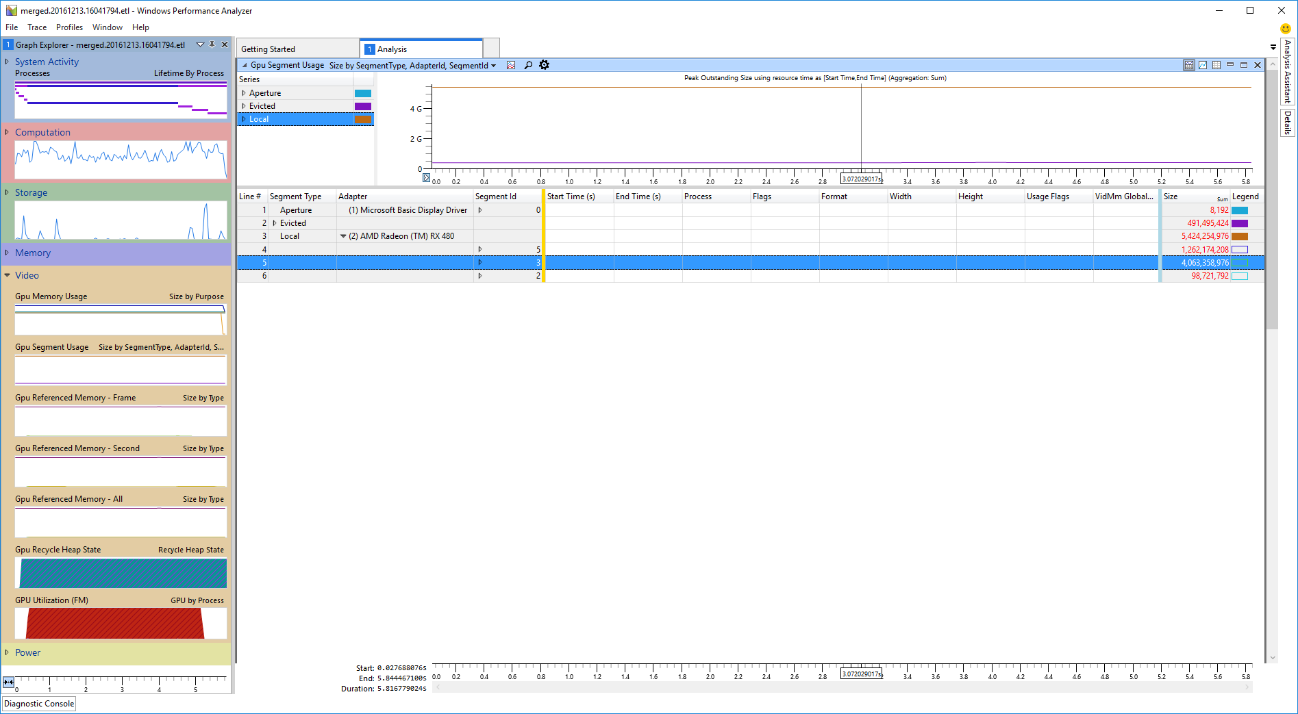
Under the graph there is a table containing video allocations. Each table line corresponds to either a video allocation or a dropdown under which allocations are grouped. Each table column corresponds to an allocation attribute. The columns are split into areas separated by colored table lines.

To the left of the yellow line, there are the attributes by which the allocations are grouped by, in order of grouping from left to right. By default, allocations are grouped first by Segment Type, second by Adapter and third by Segment Id.

To the right of the blue line are the size and legend color columns. The size column shows individual allocation sizes for allocation lines and the sum of all allocations belonging to a dropdown for the dropdown lines. The legend column displays the associated graph color of a given grouping in a solid box. If only the box outline is displayed, that means that particular grouping isn’t plotted on the graph. Clicking on the color box under the legend column will toggle the graph visibility for individual groupings.

In between the yellow and blue lines are the regular data columns, displaying the attributes of individual allocations. These columns display no information for allocation groupings.

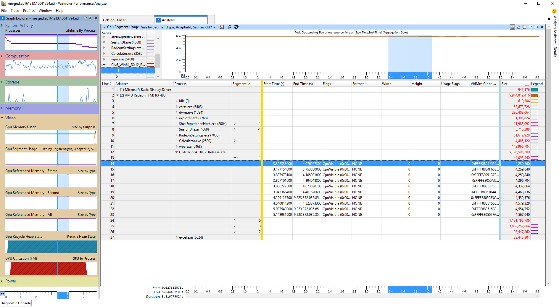
The default grouping does not work very well, but it is very easy to change. Typically a more useful grouping would be to group first by Adapter, second by Segment Type and third by Process. This can be done by dragging the columns into their proper place with the mouse. The Segment Type column can be removed by right clicking on the table header and unchecking the appropriate box.

Since the groupings are so easy to reconfigure, it helps to do so often when analyzing, in order to easily navigate the table. Another useful tip is to Filter To Selection: for example if it is apparent that processes other than the profiled app are contributing insignificantly to GPU segment usage, the groupings can be changed to Adapter, Process and Segment ID, expand the Adapter tab for the desired adapter and then right click on the target process and select Filter To Selection. This will hide every allocation that is not associated with that particular adapter and process.

Once groupings are reconfigured, the Legend tab typically needs setup to be able to display meaningful graphs.

Identifying GPU segments

For AMD, there are three GPU segments:

• Local visible, this is fixed at 256MB in size regardless of GPU. Local refers to the fact that this memory is video memory (VRAM) and visible refers to the fact that the CPU can directly access this video memory. Most of the resources in this segment are CPU_READ/WRITE flagged.
• Local invisible, the size is ASIC-specific. For example, on a Radeon RX 480 8GB card, the size will be 8GB – 256MB = 7.75GB. Invisible refers to the fact that the CPU cannot directly access this video memory. Most of an application’s graphics resources should be residing here.
• System, the size is relatively large, typically capped at about half of system memory size. This is system memory (not video memory) that can be directly accessed by the GPU. DirectX 11 staging and dynamic resources and DirectX 12 upload heap resources typically account for the most of the usage.

In addition, WPA lists evicted resources under segment ID -1. One of the reasons for resources getting evicted is when they have a specific need to be in certain segments, but there is no more space left in those segments. For instance, for some resources, various restrictions could require them to be in Local Visible when used. If too many such resources are competing for space, the video memory manager will evict some of them to free up space. This can result in thrashing patterns as the evicted resources need to be moved back in. Resources getting copied around the various segment IDs manifest as stutters/spikes in your app.

The evicted segment is the only one that is identifiable just by segment ID, as it’s always -1. The actual GPU segments are not easy to match to segment IDs, so the first step when analyzing GPU segment usage with WPA is always to identify which segment ID in a profile matches which GPU segment.

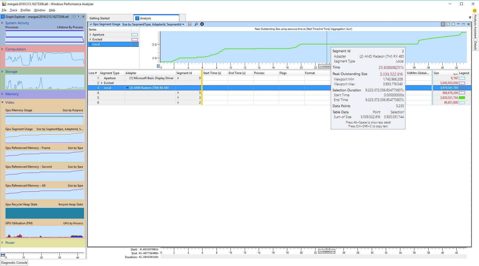
The total size of all allocations on a particular segment at a single moment in time, particularly at the peak of usage, is a very important bit of information needed in order to quickly identify the segments. However, the Size column will display the sum of all allocations across the entire time interval visible in the graph (which by default is for the life of the entire profile), so that information is not useful for understanding peak capacity. The graph actually holds the information of interest, as it charts the total allocation size across time. So to begin, for each segment ID, toggle the Legend column colors such that only individual segment get charted at a time and retrieve the size information for each segment from the graph. In case a segment sees a large variation in total capacity used, it’s the peak usage that is most interesting for identifying the segment.

Rough steps for identifying the segments are:

• Local invisible typically holds and should hold most of the resources, so the segment with the highest peak usage is the most likely to be Local invisible.
• Local visible cannot exceed 256MB of peak usage, so if two of the segments exceed that in peak usage, by exclusion the third segment has to be Local visible.
• If the system segment is under 256MB, which is common, you can check to see if one of the two unidentified segments peak usage seems to be capped just under 256MB. If that is the case, toggle the Legend column to display only that segment and Evicted (-1) and notice if there are any correlations in size changes are correlated in the two segments. If so, both Local visible and an oversubscription issue have been identified.
• If the Local visible segment is not getting oversubscribed, this means most of CPU visible flagged resources will end up here. Under the Flags column, look through the allocations on both your low usage (<256MB) segments and check for the CpuVisible The Local visible segment will typically be predominated by resources flagged as CPU visible, whereas they will be rare in the System segment. It’s important to note this will not hold if there is oversubscription of Local visible, since resources that would typically reside in Local visible could be moved to System to avoid thrashing, so the previous step needs to be followed first.

Checking for video memory oversubscription

Once the segments have been identified, the obvious thing to determine is whether any oversubscription is present. Oversubscription, in either Local Visible or Local Invisible has two negative effects: resources can end up in a suboptimal segment (for example a texture could end up being used from system instead of local, causing perf issues) and thrashing can cause stutters and spikes as the resources get copied around.

To check for stutters due to oversubscription, look at the Evicted segment and sort the allocations by the Start Time column. A number of allocations should already have been evicted when profiling begun, so the first lines in the table should display 0 as the Start Time. All the other evicted allocations have been evicted during the profiling itself. Evaluate the size and frequency of these evictions to determine if they could be an issue. If these evictions are large or happen often, look at the other segment and match the Start Time in the Evicted segment with an End Time in a source segment to find out where those resources have been evicted from. Some resources can start as evicted and then get transferred into a segment, completely unrelated to oversubscription. These typically reside in Evicted for very brief periods of time so they can be recognized by noticing the End Time and Start Time delta is very small (roughly around 0.001ms).

To check for resources ending up in suboptimal segments (like a resource that would be preferred for Local Invisible ending up in System), check if the peak usage of either of the local segments is close to capacity. If so, for Local Invisible the easiest way to confirm oversubscription is to install a GPU with higher VRAM than your app budget. For example, if you’re worried about oversubscription on a 4GB Fury X, profile on an 8GB Radeon RX 480 instead. Compare the peak usage of the System and Local Visible segments across the two cards and if the 4GB card uses more System and_/_or Local Visible (and is also close to capacity on Local Invisible), this means Local Invisible is oversubscribed on the 4GB card. If a higher VRAM capacity card is not available or if it’s Local Visible that’s close to capacity, compare the target segment’s graph with the other segments and try to find correlation in usage changes between segments (try determining it resource from the target segment are being moved to other segments or evicted).

Ultimately, check the System and Evicted segments for contents. If there is large total usage of these segments, that alone is cause for concern, since this implies either oversubscription, leaked resources, rarely used resources or other issues with the way video memory is managed. If large, the resources in those segments should be identified.

Identifying video memory resources and budgeting

The common remedy for video memory oversubscription/thrashing is to optimize the app to use less video memory. For this to be possible, it is necessary to be able to breakdown video memory usage into categories for budgeting and also to be able to identify the WPA allocations (understand what app resources they are associated with).

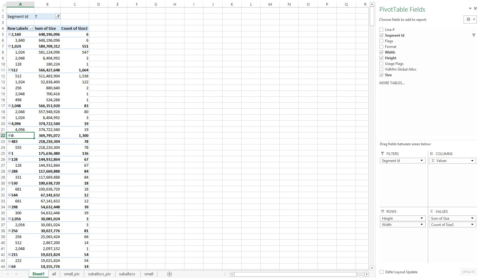
For identifying categories of resources, exporting all the allocations to a spreadsheet editor helps. In order to do so, group all the allocations needing export into a single dropdown in WPA. It’s generally useful to export all the allocations belonging to a process, so in WPA the columns can be configured such that only the Process column is left of the yellow line. To actually export, select all the allocations under the target process (shift-click), right click on them and select Copy Selection. The cells can then be pasted in a spreadsheet editor.

To get a good overview and rough breakdown of resources, create a pivot table that groups resources first by Height, then by Width. Have the pivot table count the resources in each category and also sum the resource sizes. This pivot table can be sorted by the sum of resource sizes to quickly show which the most significant resource categories are.

Chances are, the most relevant categories are:

• Resources of height 0
  • DirectX 11 suballocations, they are collections of small resources that have been grouped together by the driver under larger allocations in order to avoid wasting VRAM due to alignment restrictions. Suballocations all have the same size, usually 32KB (but this could be some other similar power of 2 size). The total suballocation size is typically significant (10-20% of overall VRAM usage). It is difficult to further analyze or optimize this category, since the actual resources are hidden behind the suballocations.
  • Shader binaries
  • Driver internal resources
  • Descriptor heaps
  • DirectX 12 placed resource heaps
• Resources of height 1, these are buffers (vertex buffers, index buffers, constant buffers, 1D textures etc)
• Textures (width/height > 1)
  • Screen sized or factors of screen size, these are likely all RTs. This category is expected to scale proportionally with screen resolution. Reusing the same RT for multiple rendering passes instead of creating dedicated RTs is a common optimization of this segment.
  • Power of 2 sized textures, this is an easy segment to quickly scan for surprises. For example, unusually high texture dimensions or texture count could be observed.
  • Non-power of 2 sized textures. For textures with mipmaps, the allocation size needs to fit the texture rounded up to the next power of 2 size. If one dimension of the texture is just over a power of 2, there will be a lot of wasted VRAM. For example, a 530/530 texture with mipmaps will occupy just as much space as a 1024/1024 texture with mipmaps. As such, for this category it’s good to make sure the total size is either insignificant or that the texture sizes are just under powers of 2. A common remedy for issues with this category is to resize the texture to the closest power of 2 (for example, resizing 530/530 textures to 512/512).

To better understand video memory usage, it’s useful to create additional pivot tables or use additional filtering (by segment, format, flags etc.) One useful example is to create a pivot table of only small resources. For DirectX 11, these can be all resources smaller than the suballocation size (usually 32KB). For DirectX 12, an arbitrary size can be chosen (or multiple sizes for additional pivot tables). Small resources should be insignificant in total size in DirectX 11, since most of them should be automatically suballocated by the driver. For DirectX 12 it is up to the app to suballocate most small resources, so this is a good way to check that the profiled allocations match expected app behavior.

Other textures may incur padding as well as non-power-of-two, especially on higher end video cards where the wide memory buses require larger alignment to deliver maximum performance – this extra padding is one of the largest differences between typical discrete GPUs and integrated and other unified memory solutions where the bus is not so wide. Keep an eye out for allocation sizes that are significantly larger than the image data. The spreadsheet table can be set up to calculate the expected size and compare this with the actual size. If there is significant waste, options for reducing this overhead include combining small textures into larger atlases and adjusting the bind flags or texture format to give the driver options to switch to smaller padding sizes (for example, a rendertarget or depth buffer is more likely to incur padding overhead than a texture). Formats with smaller texel sizes generally require less padding than those with larger sizes, with the exception of the BC formats (4bpp BC formats are equivalent to 64-bit texels, and 8bpp BC formats are equivalent to 128-bit texels).

There are many features and usage cases to WPA and this can make the tool difficult to approach. This post provides an easier introduction to this essential tool, allowing the readers to build on this knowledge to further explore on their own. I hope this has improved the understanding of both the hardware and driver model and that this knowledge will be put to good use by developers in delivering high performance graphics.