Using HIP RT ray tracing library to accelerate fluid simulation

Originally posted: November 9, 2023

Last updated: June 26, 2024

Tianchen Xu

Takahiro Harada

Introduction

HIP RT is a ray tracing library which is mostly used to accelerate ray tracing applications. However, as the library is general, it is possible to use it for applications in different fields. In this blog post, we introduce an interesting application of HIP RT for a physically-based simulation. Specifically, we show that it is possible to use HIP RT to accelerate neighbor search in Smoothed Particle Hydrodynamics (SPH) simulation [1]. Accelerating Particle-based fluid simulation using a GPU has been studied long time [2] but as you can read from this blog post, HIP RT makes it easy to implement an SPH simulation on GPUs.

In terms of the basic SPH implementation without incompressibility, the most computationally expensive process is particle neighbor search. In the various data structures for neighbor search, there are structured and unstructured organizations. A uniform grid is a typical structured organization, which divides the simulation space into uniform cells. It also indicates that the simulation space is limited by the range of the grid because it allocates memory for the entire space defined in the grid. Meanwhile, a Bounding Volume Hierarchy (BVH) is an unstructured organization. Although the search on a BVH is not generally faster than using a uniform grid [3], using a BVH has an advantage where we do not need to constrain the simulation space. Therefore, it is capable to provide much better flexibility for the cases of large-scale scenes and save memory space for sparsely distributed particles.

Here we started to see something in common in these 2 applications, BVH, the spatial acceleration data structure. Most ray tracing implementations use the BVH scheme, such as DirectX and Vulkan ray tracing (DXR and Vulkan RT). Per DXR and Vulkan RT specifications [4, 5], ray-triangle intersection can only occur if the intersection ray length t-value satisfies $T_\text{min} \lt t \lt T_{max}$ , while ray-procedural-primitive intersection can only occur if the intersection t-value satisfies $T_\text{min} \leq t \leq T_\text{max}$ . HIP RT also adopts the same rule. Hence, if we change the ray as a zero-length ray, we can use it to find an interseciton of a point to an Axis Aligned Bounding Box (AABB) which is the exact operation we need to perform in particle-based fluid simulation. After finding neighbor particles, we need to compute some physical values from them which can be implemented with custom intersection function which is also provided in HIP RT. Thus, we have all the pieces we need to implement SPH simulation using HIP RT.

About SPH fluid simulation

Smoothed Particle Hydrodynamics (SPH) is a particle-based fluid simulation method, also known as Lagrangian scheme in contrast to the Eularian grid scheme. It focuses on the dynamic attributes of each particle impacted by other particles, such as the density, force (or acceleration), velocity, and position. For each particle $i$ , the attribute quantity denoted by $A_i$ is interpolated at location $\mathbf{r}_i$ by the following model [6] in kernel-density estimation (KDE) form (a weighted sum of contributions from all particles):

A_i(\mathbf{r}_i) = \sum_j m_j \dfrac{A_j}{\rho_j}W\left(\mathbf{r}_i - \mathbf{r}_j, h\right) \tag{1}

where $j$ iterates over all particles, $m_j$ is the mass of particle $j$ , $r_j$ denotes its position, $\rho_j$ is the density, and $A_j$ the corresponding attribute quantity of particle $j$ . The function $W(\mathbf{r},h)$ is called the smoothing kernel with core radius $h$ .

According to the basic SPH model, the simulation process can be implemented in three compute passes, and each pass is a particle-traversal process.

Firstly, for each particle, we traverse all the nearby particles within radius $h$ , fetch their positions, calculates the particle distances, and evaluate the particle density value $\rho_i$ using the below KDE formula with $W = W_\text{poly6}$ :

\rho_i(\mathbf{r}_i) = \sum_j m_j \dfrac{\rho_j}{\rho_j}W\left(\mathbf{r}_i - \mathbf{r}_j, h\right) = \sum_j^{\|\mathbf{r}_i - \mathbf{r}_j\| \leq h} m_j W_\text{poly6}\left(\mathbf{r}_i - \mathbf{r}_j, h\right) \tag{2}

W_\text{poly6}(\mathbf{r}, h) = \begin{cases} \dfrac{315}{64\pi h^9}\left(h^2 - \mathbf{r}^2\right)^3 & 0 \leq \|\mathbf{r}\| \leq h\\ 0 & \text{otherwise} \end{cases} \tag{3}

Secondly, for each particle, we traverse all the nearby particles within radius $h$ , fetch their positions, pressures, and velocities, and evaluate the acceleration contributions of the pressure and viscosity terms with $W_\text{spiky}$ and $W_\text{viscosity}$ , respectively:

\mathbf{f}_i^\text{pressure}(\mathbf{r}_i) = -\sum_j^{\|\mathbf{r}_i - \mathbf{r}_j\| \leq h} m_j \dfrac{p_i + p_j}{2\rho_j} \nabla W_\text{spiky}\left(\mathbf{r}_i - \mathbf{r}_j, h\right) \tag{4}

\nabla W_\text{spiky}(\mathbf{r}, h) = \begin{cases} -\dfrac{45\mathbf{r}}{\pi h^6\|\mathbf{r}\|}\left(h - \|\mathbf{r}\|\right)^2 & 0 \leq \|\mathbf{r}\| \leq h\\ 0 & \text{otherwise} \end{cases} \tag{5}

where $p_i$ and $p_j$ denote the pressure values of particles $i$ and $j$ respectively. The pressure value $p$ can be derived from the density value by $p = k\left(\left(\frac{\rho}{\rho_0}\right)^3 - 1\right)$ , where $k$ is a gas constant that depends on the temperature and $\rho_0$ is the rest density.

\mathbf{f}_i^\text{viscosity}(\mathbf{r}_i) = \mu\sum_j^{\|\mathbf{r}_i - \mathbf{r}_j\| \leq h} m_j \dfrac{\mathbf{v}_j - \mathbf{v}_i}{\rho_j} \nabla^2 W_\text{viscosity}\left(\mathbf{r}_i - \mathbf{r}_j, h\right) \tag{6}

\nabla^2 W_\text{viscosity}(\mathbf{r}, h) = \begin{cases} \dfrac{45}{\pi h^6}\left(h - \|\mathbf{r}\|\right) & 0 \leq \|\mathbf{r}\| \leq h\\ 0 & \text{otherwise} \end{cases} \tag{7}

where $\mathbf{v}_i$ and $\mathbf{v}_j$ represent the velocity values of particles $i$ and $j$ respectively, and $\mu$ is the viscosity constant.

Finally, for each particle, we calculate the force composition from internal (pressure and diffusion) and external forces, and update the acceleration, velocity, and position according to Navier-Stokes equation:

\dfrac{\partial\mathbf{v}}{\partial t} + \mathbf{v}\cdot\nabla\mathbf{v} = -\dfrac{\nabla p}{\rho} + \dfrac{\mu}{\rho}\nabla^2\mathbf{v} + \mathbf{f}^\text{external} = \mathbf{f}^\text{pressure} + \mathbf{f}^\text{viscosity} + \mathbf{f}^\text{external} \tag{8}

where $\mathbf{f}^\text{external}$ is the acceleration contribution of the external forces. Here, symbol $\mathbf{f}$ is actually an acceleration value habitually denoted as a force in many computer graphics papers.

Using HIP RT custom intersection function to do neighbor search

As described in the last section, the major two processing passes of density and force calculations are implemented on the formula pattern of Equation (1). For each particle, we need to collect the attributes of the nearby particles within core radius $h$ by iteratively neighbor searching. For each search iteration, we seek a particle within $h$ and access its attribute data. This process is costly and to implement a fast and optimized neighbor search algorithm is not that simple. Fortunately, by taking advantage of hiprtGeomCustomTraversalAnyHit, we can iteratively access all particle attributes within our specified impact radius $h$ conveniently.

Firstly, we implement the density kernel program with HIP RT following Equation (2) for example:

extern "C" __global__ void
DensityKernel( hiprtGeometry geom, float* densities, const Particle* particles, Simulation* sim, hiprtFuncTable table )
{
    const unsigned int idx      = blockIdx.x * blockDim.x + threadIdx.x;
    Particle           particle = particles[idx];

    hiprtRay ray;
    ray.origin    = particle.Pos;
    ray.direction = { 0.0f, 0.0f, 1.0f };
    ray.minT      = 0.0f;
    ray.maxT      = 0.0f;

    hiprtGeomCustomTraversalAnyHit tr( geom, ray, hiprtTraversalHintDefault, sim, table );

    float rho = 0.0f;
    while ( tr.getCurrentState() != hiprtTraversalStateFinished )
    {
        hiprtHit hit = tr.getNextHit();
        if ( !hit.hasHit() ) continue;

        rho += calculateDensity( hit.t, sim->m_smoothRadius, sim->m_densityCoef );
    }

    densities[idx] = rho;
}

In the density kernel program, densities is an output buffer, particles is an input particle-data buffer (including particle positions and velocities), and sim is a constant buffer of simulation parameters. Here, we first set hiprtRay with a zero-length ray in an arbitrary normalized direction, whose ray.minT = ray.maxT = 0. Then, we interactively access the hit results until the any hit state is hiprtTraversalStateFinished. For safety, we skip the miss iteration explicitly. For each iteration, we calculate the density following Equations (2, 3) by calling calculateDensity:

__device__ float calculateDensity( float r2, float h, float densityCoef )
{
  // Implements this equation:
  // W_poly6(r, h) = 315 / (64 * pi * h^9) * (h^2 - r^2)^3
  // densityCoef = particleMass * 315.0f / (64.0f * pi * h^9)
  const float d2 = h * h - r2;

  return densityCoef * d2 * d2 * d2;
}

For hiprtGeomCustomTraversalAnyHit, we also need to design a custom intersection function stored in hiprtFuncTable and called by getNextHit implicitly:

__device__ bool intersectParticleImpactSphere( const hiprtRay& ray, const void* data, void* payload, hiprtHit& hit )
{
    float3      from     = ray.origin;
    Particle    particle = reinterpret_cast<const Particle*>( data )[hit.primID];
    Simulation* sim      = reinterpret_cast<Simulation*>( payload );
    float3      center   = particle.Pos;
    float       h        = sim->m_smoothRadius;

    float3 d  = center - from;
    float  r2 = dot( d, d );
    if ( r2 >= h * h ) return false;

    hit.t      = r2;
    hit.normal = d;

    return true;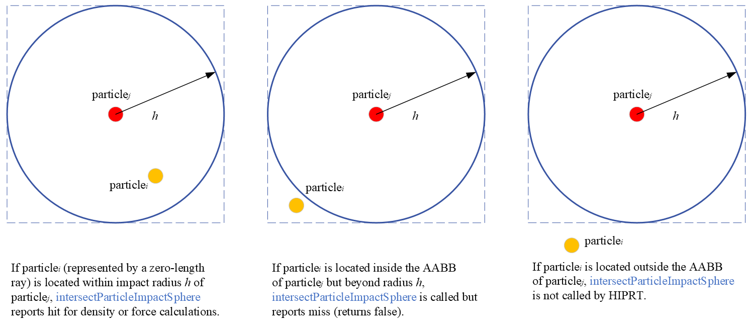
}

In intersectParticleImpactSphere, we obtain the ray origin as the position of particle $i$ and the position of particle $j$ and cull the particle beyond impact radius $h$ by spherical checking. Then, we leverage t (the current ray length) and normal slots to store the values of square distance r2 and displacement vector d into the hit object respectively and pass them to the main kernel program. They will be used for the later density and force calculations.

For the second simulation pass, we have a similar kernel program for force evaluations:

extern "C" __global__ void ForceKernel(
  hiprtGeometry  geom,
  float3*         accelerations,
  const Particle* particles,
  const float*  densities,
  Simulation*     sim,
  hiprtFuncTable  table )
{
  const unsigned int idx      = blockIdx.x * blockDim.x + threadIdx.x;
  Particle           particle = particles[idx];
  float              rho      = densities[idx];

  hiprtRay ray;
  ray.origin    = particle.Pos;
  ray.direction = { 0.0f, 0.0f, 1.0f };
  ray.minT      = 0.0f;
  ray.maxT      = 0.0f;

  float pressure = calculatePressure( rho, sim->m_restDensity, sim->m_pressureStiffness );

  hiprtGeomCustomTraversalAnyHit tr( geom, ray, hiprtTraversalHintDefault, sim, table );

  float3 force = make_float3( 0.0f );
  while ( tr.getCurrentState() != hiprtTraversalStateFinished )
  {
    hiprtHit hit = tr.getNextHit();
    if ( !hit.hasHit() ) continue;
    if ( hit.primID == idx ) continue;

    Particle hitParticle = particles[hit.primID];
    float   hitRho      = densities[hit.primID];

    float3 disp        = hit.normal;
    float  r           = sqrtf( hit.t );
    float  d           = sim->m_smoothRadius - r;
    float  hitPressure = calculatePressure( hitRho, sim->m_restDensity, sim->m_pressureStiffness );

    force += calculateGradPressure( r, d, pressure, hitPressure, hitRho, disp, sim->m_pressureGradCoef );
    force += calculateVelocityLaplace( d, particle.Velocity, hitParticle.Velocity, hitRho, sim->m_viscosityLaplaceCoef );
  }

  accelerations[idx] = rho > 0.0f ? force / rho : make_float3( 0.0f );
}

ForceKernel is to evaluate the acceleration contribution of particle $i$ from the internal forces, which has the same code pattern to DensityKernel. Here, we skip the calculation for the hit of particle $j$ when $i = j$ to avoid redundant data accesses and calculations for performance optimization. Besides, we use the same custom intersection function to the density kernel. Additionally, the functions to calculate the pressure, pressure gradient, and viscous term, based on Equations (4–7), are implemented as follows:

__device__ float calculatePressure( float rho, float rho0, float pressureStiffness )
{
  // Implements this equation:
  // Pressure = B * ((rho / rho_0)^3 - 1)
  const float rhoRatio = rho / rho0;

  return pressureStiffness * max( rhoRatio * rhoRatio * rhoRatio - 1.0f, 0.0f );
}

__device__ float3
calculateGradPressure( float r, float d, float pressure, float pressure_j, float rho_j, float3 disp, float pressureGradCoef )
{
  float avgPressure = 0.5 * ( pressure + pressure_j );
  // Implements this equation:
  // W_spiky(r, h) = 15 / (pi * h^6) * (h - r)^3
  // GRAD(W_spiky(r, h)) = -45 / (pi * h^6) * (h - r)^2
  // pressureGradCoef = particleMass * -45.0f / (pi * h^6)

  return pressureGradCoef * avgPressure * d * d * disp / ( rho_j * r );
}

__device__ float3
calculateVelocityLaplace( float d, float3 velocity, float3 velocity_j, float rho_j, float viscosityLaplaceCoef )
{
  float3 velDisp = ( velocity_j - velocity );
  // Implements this equation:
  // W_viscosity(r, h) = 15 / (2 * pi * h^3) * (-r^3 / (2 * h^3) + r^2 / h^2 + h / (2 * r) - 1)
  // LAPLACIAN(W_viscosity(r, h)) = 45 / (pi * h^6) * (h - r)
  // viscosityLaplaceCoef = particleMass * viscosity * 45.0f / (pi * h^6)

  return viscosityLaplaceCoef * d * velDisp / rho_j;
}

For the final simulation pass, we compose an integration kernel program to calculate the force composition from internal and external forces of each particle, and update the acceleration, velocity, position, and AABB according to Equation (8):

extern "C" __global__ void IntegrationKernel(
  Particle* particles, Aabb* particleAabbs, const float3* accelerations, const Simulation* sim, const PerFrame* perFrame )
{
  const unsigned int idx          = blockIdx.x * blockDim.x + threadIdx.x;
  Particle           particle     = particles[idx];
  float3             acceleration = accelerations[idx];

  // Apply the forces from the map walls
  for ( u32 i = 0; i < 6; ++i )
  {
    float d       = dot( make_float4( particle.Pos, 1.0f ), sim->m_planes[i] );
    acceleration += min( d, 0.0f ) * -sim->m_wallStiffness * make_float3( sim->m_planes[i] );
  }

  // Apply gravity
  acceleration      += perFrame->m_gravity;

  // Integrate
  particle.Velocity += perFrame->m_timeStep * acceleration;
  particle.Pos      += perFrame->m_timeStep * particle.Velocity;

  Aabb aabb;
  aabb.m_min = particle.Pos - sim->m_smoothRadius;
  aabb.m_max = particle.Pos + sim->m_smoothRadius;

  // Update
  particles[idx]     = particle;
  particleAabbs[idx] = aabb;
}

Based on the acceleration value of the internal forces computed in the last pass, we deploy a simple boundary condition model that reflects the particle motion from the hit wall according to the wall plane and stiffness parameter m_wallStiffness, and accumulate the reflection as an external force contribution to the acceleration value. Also, we need to add the gravity contribution. Using this resultant acceleration, we can easily derive the new velocity, position, and AABB values in sequence.

Host-side implementation with HIP RT

Firstly, we define two structures for buffers Simulation and Particle to store the necessary input parameters and particle data:

struct Simulation
{
    float  m_smoothRadius;
    float  m_pressureStiffness;
    float  m_restDensity;
    float  m_densityCoef;
    float  m_pressureGradCoef;
    float  m_viscosityLaplaceCoef;
    float  m_wallStiffness;
    u32    m_particleCount;
    float4 m_planes[6];
};

struct Particle
{
    float3 Pos;
    float3 Velocity;
};

We populate the initial data of these two buffers for the scenario described as below:

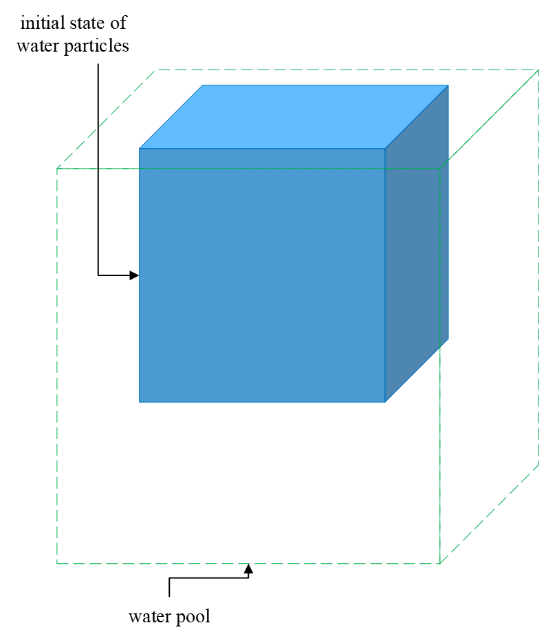
In a cubic water pool of $1 \ \mathrm{m}^3$ , water particles fall from the pool ceil. The initial shape of the water volume is a cube of $0.216 \ \mathrm{m}^3$ . Water particles are uniformly distributed in the water volume, and the number of particles is specified as $131,072$ . For other parameters, please refer to the property of water, such as the rest density $1000 \left.\mathrm{kg}\middle/\mathrm{m}^3\right.$ and particle mass derived from the aforementioned conditions. The viscosity value is $0.4$ . The stiffness value of all pool walls is $3000$ . The particle search radius is specified as $0.02 \ \mathrm{m}$ , i.e., SPH smoothing radius $h$ .

Subsequently, a very important step for ray tracing is to build an acceleration structure (AS). Here, we choose hiprtGeometry which has the bottom-level AS only for convenience. We use hiprtPrimitiveTypeAABBList as the type of the corresponding hiprtGeometryBuildInput. For each AABB element, we populate the initial data based on the initial particle positions:

hiprtAABBListPrimitive list;
list.aabbCount  = sim.m_particleCount;
list.aabbStride = sizeof( Aabb );
std::vector<Aabb> aabbs( sim.m_particleCount );
for ( u32 i = 0; i < sim.m_particleCount; ++i )
{
    const hiprtFloat3& c = particles[i].Pos;
    aabbs[i].m_min.x     = c.x - smoothRadius;
    aabbs[i].m_max.x     = c.x + smoothRadius;
    aabbs[i].m_min.y     = c.y - smoothRadius;
    aabbs[i].m_max.y     = c.y + smoothRadius;
    aabbs[i].m_min.z     = c.z - smoothRadius;
    aabbs[i].m_max.z     = c.z + smoothRadius;
}

Since the particle AABBs can be updated per frame, we choose hiprtBuildFlagBitPreferFastBuild mode to build the acceleration structure and will rebuild the entire hiprtGeometry each frame.

hiprtGeometryBuildInput geomInput;
geomInput.type               = hiprtPrimitiveTypeAABBList;
geomInput.aabbList.primitive = list;
geomInput.geomType           = 0;

size_t            geomTempSize;
hiprtDevicePtr    geomTemp;
hiprtBuildOptions options;
options.buildFlags = hiprtBuildFlagBitPreferFastBuild;
CHECK_HIPRT( hiprtGetGeometryBuildTemporaryBufferSize( ctxt, geomInput, options, geomTempSize ) );
CHECK_ORO( oroMalloc( reinterpret_cast<oroDeviceptr*>( &geomTemp ), geomTempSize ) );

hiprtGeometry geom;
CHECK_HIPRT( hiprtCreateGeometry( ctxt, geomInput, options, geom ) );

Here, you see oro functions which are functions of Orochi library which wraps HIP and CUDA APIs. Therefore, the code written with Orochi should run on non-AMD GPU too.

Then, we register the function table for the custom intersection function. As aforementioned, we use the same intersection function intersectParticleImpactSphere for both the density and force kernel programs.

hiprtFuncNameSet funcNameSet;
funcNameSet.intersectFuncName              = "intersectParticleImpactSphere";
std::vector<hiprtFuncNameSet> funcNameSets = { funcNameSet };

hiprtFuncDataSet funcDataSet;
CHECK_ORO( oroMalloc(
    reinterpret_cast<oroDeviceptr*>( &funcDataSet.intersectFuncData ),
    sim.m_particleCount * sizeof( Particle ) ) );
CHECK_ORO( oroMemcpyHtoD(
    reinterpret_cast<oroDeviceptr>( funcDataSet.intersectFuncData ),
    particles.data(),
    sim.m_particleCount * sizeof( Particle ) ) );

hiprtFuncTable funcTable;
CHECK_HIPRT( hiprtCreateFuncTable( ctxt, 1, 1, funcTable ) );
CHECK_HIPRT( hiprtSetFuncTable( ctxt, funcTable, 0, 0, funcDataSet ) );

After setting the function table, we can build the kernel programs of the three simulation passes accordingly. We allocate the corresponding output buffer of each pass by the way.

// Density
float*      densities;
oroFunction densityFunc;
CHECK_ORO( oroMalloc( reinterpret_cast<oroDeviceptr*>( &densities ), sim.m_particleCount * sizeof( float ) ) );
buildTraceKernelFromBitcode(
    ctxt, "../common/TutorialKernels.h", "DensityKernel", densityFunc, nullptr, &funcNameSets, 1, 1 );

// Force
hiprtFloat3* accelerations;
oroFunction  forceFunc;
CHECK_ORO(
    oroMalloc( reinterpret_cast<oroDeviceptr*>( &accelerations ), sim.m_particleCount * sizeof( hiprtFloat3 ) ) );
buildTraceKernelFromBitcode(
    ctxt, "../common/TutorialKernels.h", "ForceKernel", forceFunc, nullptr, &funcNameSets, 1, 1 );

// Integration
PerFrame*  pPerFrame;
oroFunction intFunc;
{
    PerFrame perFrame;
    perFrame.m_timeStep = 1.0f / 320.0f;
    perFrame.m_gravity  = { 0.0f, -9.8f, 0.0f };
    CHECK_ORO( oroMalloc( reinterpret_cast<oroDeviceptr*>( &pPerFrame ), sizeof( PerFrame ) ) );
    CHECK_ORO( oroMemcpyHtoD( reinterpret_cast<oroDeviceptr>( pPerFrame ), &perFrame, sizeof( PerFrame ) ) );
    buildTraceKernelFromBitcode( ctxt, "../common/TutorialKernels.h", "IntegrationKernel", intFunc );
}

Finally, we can construct a main simulation loop to dispatch the HIP RT kernels in order. For each frame iteration, we first rebuild the HIP RT geometry for AS updating, and then launch the kernel programs with the pointers of the required buffers put in the entry-point arguments of the kernels.

const u32 b   = 64; // Thread block size
u32       nb = ( sim.m_particleCount + b - 1 ) / b; // Number of blocks

// ...

// Simulate
for ( u32 i = 0; i < FrameCount; ++i )
{
    CHECK_HIPRT( hiprtBuildGeometry( ctxt, hiprtBuildOperationBuild, geomInput, options, geomTemp, 0, geom ) );

    void* dArgs[] = { &geom, &densities, &funcDataSet.intersectFuncData, &pSim, &funcTable };
    CHECK_ORO( oroModuleLaunchKernel( densityFunc, nb, 1, 1, b, 1, 1, 0, 0, dArgs, 0 ) );

    void* fArgs[] = { &geom, &accelerations, &funcDataSet.intersectFuncData, &densities, &pSim, &funcTable };
    CHECK_ORO( oroModuleLaunchKernel( forceFunc, nb, 1, 1, b, 1, 1, 0, 0, fArgs, 0 ) );

    void* iArgs[] = { &funcDataSet.intersectFuncData, &list.aabbs, &accelerations, &pSim, &pPerFrame };
    CHECK_ORO( oroModuleLaunchKernel( intFunc, nb, 1, 1, b, 1, 1, 0, 0, iArgs, 0 ) );

    // ...
}

Conclusion

HIP RT has similar functionality as DXR and Vulkan RT, and provides an easier and more flexible alternative to implement the point queries for neighbor search used in fluid simulation, by taking advantage of the fast dynamic geometry acceleration structure update and custom intersection function. The BVH traversal of neighbor search can be automatically and implicitly done by HIP RT efficiently. We recently released the new version of HIP RT (v.2.1) where we added more functionalities. We would like to hear if you have an interesting use case of HIP RT.

This sample has been included in the HIP RT SDK tutorials (https://github.com/GPUOpen-LibrariesAndSDKs/HIPRTSDK).

The code of kernel programs: https://github.com/GPUOpen-LibrariesAndSDKs/HIPRTSDK/blob/main/tutorials/common/TutorialKernels.h
The host-side C++ code: https://github.com/GPUOpen-LibrariesAndSDKs/HIPRTSDK/blob/main/tutorials/14_fluid_simulation/main.cpp
Some related data structures defined: https://github.com/GPUOpen-LibrariesAndSDKs/HIPRTSDK/blob/main/tutorials/common/FluidSimulation.h

References

R. A. Gingold, J. J. Monaghan, Smoothed particle hydrodynamics: theory and application to non-spherical stars, Monthly Notices of the Royal Astronomical Society, Volume 181, Issue 3, December 1977, Pages 375–389, https://doi.org/10.1093/mnras/181.3.375
Takahiro Harada; Seiichi Koshizuka; Yoichiro Kawaguchi (2007). Smoothed particle hydrodynamics on GPUs. Computer Graphics International. pp. 63–70.
Tianchen Xu; Wen Wu; Enhua Wu (2014). Real-time generation of smoothed-particle hydrodynamics-based special effects in character animation. Computer Animations and Virtual Worlds, 25: 185–198.
DirectX Raytracing (DXR) Functional Spec, https://microsoft.github.io/DirectX-Specs/d3d/Raytracing.html
Vulkan 1.3 specification, https://registry.khronos.org/vulkan/specs/1.3/html/
Matthias Müller, David Charypar, and Markus Gross. 2003. Particle-based fluid simulation for interactive applications. In Proceedings of the 2003 ACM SIGGRAPH/Eurographics symposium on Computer animation (SCA ‘03). Eurographics Association, Goslar, DEU, 154–159, https://matthias-research.github.io/pages/publications/sca03.pdf