Jacobi Solver with HIP and OpenMP offloading

The Jacobi method serves as a fundamental iterative linear solver for Partial Differential Equations (PDE) governing a wide variety of physics of interest in high performance computing (HPC) applications. Discretization of a PDE by a numerical method, e.g. finite difference, finite volume, finite element, or any other methods, leads to a large sparse systems of equations. A stationary iterative method, such as the Jacobi, can take advantage of modern heterogeneous hierarchical systems with CPU and GPUs as it is more amenable to parallelization and require less memory compared to traditional direct methods. Jacobi iteration involves a lot of repeated matrix-vector product operations, and to a great extent limits communication between all components at every iteration. This makes Jacobi methods more favorable for GPU offloading.

In this blog, we explore GPU offloading using HIP and OpenMP target directives and discuss their relative merits in terms of implementation efforts and performance.

Note: While most HPC applications today use Message Passing Interface (MPI) for distributed memory parallelism, in this blog post we consider only a single process implementation of the Jacobi method for a demonstration purpose.

Jacobi Iterative Methods

To discuss the Jacobi iterative method, we consider a PDE with Dirichlet boundary conditions on a two dimensional domain, with spatial coordinates $x$ and $y$ , to solve Poisson’s equation: $-\nabla^2 u(x,y) = f$ , which is a generalized Laplacian. Here, $u(x,y)$ is a smooth function in the domain. The equations are discretized using finite difference method[1] in a Cartesian coordinates with a 5-point stencil:

\frac{-u_{i-1,j } + 2u_{i,j} - u_{i+1,j }}{\Delta x^2} + \frac{-u_{i, j-1} + 2u_{i,j} - u_{i, j+1}}{\Delta y^2} = f_{i,j}

The above finite difference Laplacian operator leads to a sparse matrix operator, $A$ on the vector of unknown $\bf u$ : $A {\bf u} = f$ . Here:

{\bf u} = [u_{1,1}, u_{1,2}, \cdots, u_{2,1}, \cdots, u_{i,j}, \cdots u_{n_i,n_j}].

If the matrix is decomposed into the diagonal ( $D$ ), lower ( $L$ ) and upper ( $U$ ) parts ( $A = [D + L + U]$ ), the Jacobi iterative method can be represented as:

{\bf u}^{k+1} = {\bf u}^{k} + D^{-1} \left( {\bf f} - A {\bf u}^k \right)

Here, $k$ refers to the iteration number. The values of ${\bf u}^{(k=0)}$ are the Initial Conditions.

Jacobi Code structure

The main components of the serial (CPU) Jacobi solver are:

Setup Jacobi object
- CreateMesh()
- InitializeData()
Execute Jacobi method
- Laplacian()
- BoundaryConditions()
- Update()
- Norm()

The following code shows the Jacobi solver program. In the code, Jacobi_t Jacobi(mesh); does the Jacobi object setup and Jacobi.Run() does the Jacobi solver execution.

Copied!

int main(int argc, char ** argv)
{
  mesh_t mesh;

  // Extract topology and domain dimensions from the command-line arguments
  ParseCommandLineArguments(argc, argv, mesh);

  Jacobi_t Jacobi(mesh);
  Jacobi.Run();

  return STATUS_OK;
}

Setup Jacobi Object

The Jacobi object consists of two main components:

Setup Jacobi object
- CreateMesh()
- InitializeData()

The routine CreateMesh() creates a two-dimensional Cartesian mesh with uniform mesh spacing – see Figure 1. The routine InitializeData() initializes host variables $\bf u$ (h_U in the code), the matrix-vector product $A{\bf u}$ (h_AU), the right-hand side vector $f$ (h_RHS), and the residual vector $f-A{\bf u}$ (h_RES). It also applies boundary conditions for these variables.

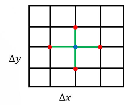
Figure 1: A uniform rectangular grid to discretize the computational domain

Execute Jacobi Method

The main Jacobi solver execution includes the following functions:

Execute Jacobi method
- Laplacian()
- BoundaryConditions()
- Update()
- Norm()

The following code shows the order of the function calls in each Jacobi iteration

Copied!

  // Scalar factor used in Jacobi method
  const dfloat factor = 1/(2.0/(mesh.dx*mesh.dx) + 2.0/(mesh.dy*mesh.dy));
  const dfloat _1bydx2 = 1.0/(mesh.dx*mesh.dx);
  const dfloat _1bydy2 = 1.0/(mesh.dy*mesh.dy);

  while ((iterations < JACOBI_MAX_LOOPS) && (residual > JACOBI_TOLERANCE))
  {
    // Compute Laplacian
    Laplacian(mesh, _1bydx2, _1bydy2, h_U, h_AU);

    // Apply Boundary Conditions
    BoundaryConditions(mesh, _1bydx2, _1bydy2, h_U, h_AU);

    // Update the solution
    Update(mesh, factor, h_RHS, h_AU, h_RES, h_U);

    // Compute residual = ||U||
    residual = Norm(mesh, h_RES);

    ++iterations;
  }

The function Laplacian() performs the main Laplacian operation discussed earlier and is shown below:

Copied!

// AU_i,j = (-U_i+1,j + 2U_i,j - U_i-1,j)/dx^2 +
//          (-U_i,j+1 + 2U_i,j - U_i,j-1)/dy^2
void Laplacian(mesh_t& mesh,
               const dfloat _1bydx2,
               const dfloat _1bydx2,
               const dfloat * U,
               dfloat * AU) {
  int stride = mesh.Nx;
  int localNx = mesh.Nx - 2;
  int localNy = mesh.Ny - 2;

  for (int j=0;j<localNy;j++) {
    for (int i=0;i<localNx;i++) {

      const int id = (i+1) + (j+1)*stride;

      const int id_l = id - 1;
      const int id_r = id + 1;
      const int id_d = id - stride;
      const int id_u = id + stride;

      AU[id] = (-U[id_l] + 2*U[id] - U[id_r])/(dx*dx) +
               (-U[id_d] + 2*U[id] - U[id_u])/(dy*dy);
    }
  }
}

The BoundaryConditions() is a function to apply boundary conditions to $A{\bf u}$ term. It applies only to the boundary nodes:

Copied!

void BoundaryConditions(mesh_t& mesh,
                        const dfloat _1bydx2,
                        const dfloat _1bydy2,
                        dfloat* U,
                        dfloat* AU) {

  const int Nx = mesh.Nx;
  const int Ny = mesh.Ny;

  for (int id=0;id<2*Nx+2*Ny-2;id++) {

    //get the (i,j) coordinates of node based on how large id is
    int i, j;
    if (id < Nx) { //bottom
      i = id;
      j = 0;
    } else if (id<2*Nx) { //top
      i = id - Nx;
      j = Ny-1;
    } else if (id < 2*Nx + Ny-1) { //left
      i = 0;
      j = id - 2*Nx + 1;
    } else { //right
      i = Nx-1;
      j = id - 2*Nx - Ny + 2;
    }

    const int iid = i+j*Nx;

    const dfloat U_d = (j==0)    ?  0.0 : U[iid - Nx];
    const dfloat U_u = (j==Ny-1) ?  0.0 : U[iid + Nx];
    const dfloat U_l = (i==0)    ?  0.0 : U[iid - 1];
    const dfloat U_r = (i==Nx-1) ?  0.0 : U[iid + 1];

     AU[iid] = (-U_l + 2*U[iid] - U_r)*_1bydx2 +
               (-U_d + 2*U[iid] - U_u)*_1bydy2;
  }
}

The essence of Jacobi solver is in the Update() function which performs the Jacobi iteration:

Copied!

//Jacobi iterative method
// U = U + D^{-1}*(RHS - AU)

void Update(mesh_t& mesh,
            const dfloat factor,
            dfloat* RHS,
            dfloat* AU,
            dfloat* RES,
            dfloat* U) 
{
  const int N = mesh.N;

  for (int id=0;id<N;id++) 
  {
    const dfloat r_res = RHS[id] - AU[id];
    RES[id] = r_res;
    U[id] += r_res*factor;
  }
}

The function Norm() is the main function that performs a reduction operation and returns a scalar residual used to check for solver convergence:

Copied!

dfloat Norm(mesh_t& mesh, dfloat *U) {

  dfloat norm = 0;
  const int N = mesh.N;
  const dfloat dx = mesh.dx;
  const dfloat dy = mesh.dy;

  for (int id=0; id < N; id++) {
    *norm2 += U[id] * U[id] * dx * dy;
  }
  return sqrt(norm)/N;
}

The next two sections describe two possible ways to port this solver onto GPUs.

GPU offload using HIP

First, we considered HIP porting for offloading the Jacobi solver to GPU. We wrote HIP kernels to port the four major code regions discussed above. Note that, for the most optimized performance, we used a launch bound of 256 (BLOCK_SIZE) for all kernels. The following code snippet shows the function calls in each Jacobi iteration, which is same as the serial code:

Copied!

  // Scalar factor used in Jacobi method
  const dfloat factor = 1/(2.0/(mesh.dx*mesh.dx) + 2.0/(mesh.dy*mesh.dy));
  const dfloat _1bydx2 = 1.0/(mesh.dx*mesh.dx);
  const dfloat _1bydy2 = 1.0/(mesh.dy*mesh.dy);

  auto timerStart = std::chrono::high_resolution_clock::now();

  while ((iterations < JACOBI_MAX_LOOPS) && (residual > JACOBI_TOLERANCE)) 
  {
    // Compute Laplacian
    Laplacian(mesh, _1bydx2, _1bydy2, HD_U, HD_AU);

    // Apply Boundary Conditions
    BoundaryConditions(mesh, _1bydx2, _1bydy2, HD_U, HD_AU);

    // Update the solution
    Update(mesh, factor, HD_RHS, HD_AU, HD_RES, HD_U);

    // Compute residual = ||U||
    residual = Norm(mesh, HD_RES);
    
    ++iterations;
  }

Some of the kernel launch configurations are set up in InitializeData(), as shown in the following code snippet:

Copied!

  // ...
  // Kernel launch configurations
  mesh.block.x = BLOCK_SIZE;
  mesh.grid.x = std::ceil(static_cast<double>(mesh.Nx * mesh.Ny) / mesh.block.x);
  mesh.grid2.x = std::ceil((2.0*mesh.Nx+2.0*mesh.Ny-2.0)/mesh.block.x);
  // ...

The code for LaplacianKernel() and Laplacian() routine that launches this kernel are shown below:

Copied!

__global__
__launch_bounds__(BLOCK_SIZE)
void LaplacianKernel(const int localNx,
                     const int localNy,
                     const int stride,
                     const dfloat fac_dx2,
                     const dfloat fac_dy2,
                     const dfloat * U,
                     dfloat * AU) 
{
    int tid = GET_GLOBAL_ID_0;

    if (tid > localNx + localNy * stride || tid < stride + 1)
        return;

    const int tid_l = tid - 1;
    const int tid_r = tid + 1;
    const int tid_d = tid - stride;
    const int tid_u = tid + stride;

    __builtin_nontemporal_store((-U[tid_l] + 2*U[tid] - U[tid_r])*fac_dx2 + 
                                (-U[tid_d] + 2*U[tid] - U[tid_u])*fac_dy2, &(AU[tid]));
}

void Laplacian(mesh_t& mesh,
               const dfloat _1bydx2,
               const dfloat _1bydy2,
               dfloat* U,
               dfloat* AU) 
{
  int stride = mesh.Nx;
  int localNx = mesh.Nx-2;
  int localNy = mesh.Ny-2;

  LaplacianKernel<<<mesh.grid,mesh.block>>>(localNx, localNy, stride, _1bydx2, _1bydy2, U, AU);
}

The kernel BoundaryConditionsKernel(), and its launching function are shown below:

Copied!

__global__
__launch_bounds__(BLOCK_SIZE)
void BoundaryConditionsKernel(const int Nx,
                              const int Ny,
                              const int stride,
                              const dfloat fac_dx2,
                              const dfloat fac_dy2,
                              const dfloat * U,
                              dfloat * AU) 
{
    const int id = GET_GLOBAL_ID_0;

    if (id < 2*Nx+2*Ny-2)
    {
	//get the (i,j) coordinates of node based on how large id is
	int i = Nx-1;
	int j = id - 2*Nx - Ny + 2;

	if (id < Nx) 
	{ //bottom
	    i = id; j = 0;
	}
	else if (id<2*Nx) 
	{ //top
	    i = id - Nx; j = Ny-1;
	}
	else if (id < 2*Nx + Ny-1) 
	{ //left
	    i = 0; j = id - 2*Nx + 1;
	}

	const int iid = i+j*stride;

	const dfloat U_d = (j==0)    ?  0.0 : U[iid - stride];
	const dfloat U_u = (j==Ny-1) ?  0.0 : U[iid + stride];
	const dfloat U_l = (i==0)    ?  0.0 : U[iid - 1];
	const dfloat U_r = (i==Nx-1) ?  0.0 : U[iid + 1];

	__builtin_nontemporal_store((-U_l + 2*U[iid] - U_r)*fac_dx2 +
                                    (-U_d + 2*U[iid] - U_u)*fac_dy2, &(AU[iid]));
    }
}

void BoundaryConditions(mesh_t& mesh,
                        const dfloat _1bydx2,
                        const dfloat _1bydy2,
                        dfloat* U,
                        dfloat* AU) {

  const int Nx = mesh.Nx;
  const int Ny = mesh.Ny;
  BoundaryConditionsKernel<<<mesh.grid2,mesh.block>>>(Nx, Ny, Nx, _1bydx2, _1bydy2, U, AU);
}

The following code shows the HIP implementation of UpdateKernel():

Copied!

__global__
__launch_bounds__(BLOCK_SIZE)
void UpdateKernel(const int N,
                  const dfloat factor,
                  const dfloat *__restrict__ RHS,
                  const dfloat *__restrict__ AU,
                  dfloat *__restrict__ RES,
                  dfloat *__restrict__ U)
{
    int tid = GET_GLOBAL_ID_0;
    dfloat r_res;
    for (int i = tid; i < N; i += gridDim.x * blockDim.x)
    {
        r_res = RHS[i] - AU[i];
        RES[i] = r_res;
        U[i] += r_res*factor;
    }
}

void Update(mesh_t& mesh,
            const dfloat factor,
            dfloat* RHS,
            dfloat* AU,
            dfloat* RES,
            dfloat* U) 
{
  UpdateKernel<<<mesh.grid,mesh.block>>>(mesh.N, factor, RHS, AU, RES, U);
}

The following code shows the HIP implementation of NormKernel() which is loosely based off the HIP dot implementation in BabelStream:

Copied!

#define NORM_BLOCK_SIZE 512
#define NORM_NUM_BLOCKS 256
__global__
__launch_bounds__(NORM_BLOCK_SIZE)
void NormKernel(const dfloat * a, dfloat * sum, int N)
{
  __shared__ dfloat smem[NORM_BLOCK_SIZE];

  int i = GET_GLOBAL_ID_0;
  const size_t si = GET_LOCAL_ID_0;

  smem[si] = 0.0;
  for (; i < N; i += NORM_BLOCK_SIZE * NORM_NUM_BLOCKS)
    smem[si] += a[i] * a[i];

  for (int offset = NORM_BLOCK_SIZE >> 1; offset > 0; offset >>= 1)
  {
    __syncthreads();
    if (si < offset) smem[si] += smem[si+offset];
  }

  if (si == 0)
    sum[GET_BLOCK_ID_0] = smem[si];
}

void NormSumMalloc(mesh_t &mesh)
{
  hipHostMalloc(&mesh.norm_sum, NORM_NUM_BLOCKS*sizeof(dfloat), hipHostMallocNonCoherent);
}

dfloat Norm(mesh_t& mesh, dfloat *U) 
{
  dfloat norm = 0.0;
  const int N = mesh.N;
  const dfloat dx = mesh.dx;
  const dfloat dy = mesh.dy;
  NormKernel<<<NORM_NUM_BLOCKS,NORM_BLOCK_SIZE>>>(U, mesh.norm_sum, N);
  hipDeviceSynchronize();
  for (int id=0; id < NORM_NUM_BLOCKS; id++)
    norm += mesh.norm_sum[id];
  return sqrt(norm*dx*dy)*mesh.invNtotal;
}

Note that the buffer mesh.norm_sum is non-coherent pinned memory, meaning that it is mapped into the address space of the GPU. We defer all interested readers to this article for a more thorough discussion. The parameters NORM_BLOCK_SIZE and NORM_NUM_BLOCKS can and should be tuned to optimize the performance on your hardware.

The Table summarizes time per iteration spent in the major kernels of the Jacobi solver with HIP porting. The grid size is $4096\times 4096$ . The total wall clock time over a $1000$ iterations is $858$ ms and achieves a compute performance of $332$ GFLOP/s on one GCD of a MI250 GPU. The most expensive code region is the Jacobi Update() routine.

Kernels	Avg Time (ms)	Percentage
Update	0.51	60.9
Laplacian	0.22	25.7
Norm	0.10	12.3
BoundaryConditions	0.01	0.9

GPU offload using OpenMP

In this section, we explore OpenMP offloading. We consider both structured and unstructured target data mapping approaches. The clang++ compiler with -fopenmp flag is used to build the openmp target offload regions. More details can be found in codes/Makefile. For example, the following command shows how to compile the Jacobi.cpp file:

Copied!

/opt/rocm/llvm/bin/clang++ -Ofast -g -fopenmp --offload-arch=gfx90a -c Jacobi.cpp -o Jacobi.o

Structured Target Data Map

Let’s consider the most expensive code region observed in the HIP ported Jacobi solver, Update(). A simple OpenMP target offload approach would be as follows:

Copied!

void Update(mesh_t& mesh,
            const dfloat factor,
            dfloat* RHS,
            dfloat* AU,
            dfloat* RES,
            dfloat* U) 
{
  const int N = mesh.N;
  #pragma omp target data map(to:RHS[0:N],AU[0:N]) map(from:RES[0:N]) map(tofrom:U[0:N])
  #pragma omp target teams distribute parallel for
  for (int id=0;id<N;id++) 
  {
    const dfloat r_res = RHS[id] - AU[id];
    RES[id] = r_res;
    U[id] += r_res*factor;
  }
}

The state variables are mapped onto device region and Jacobi update is invoked in the target region. This is an example of structured target mapping construct. Similar stuctured target mapping is done for Laplacian and Norm routines.

Copied!

void Laplacian(mesh_t& mesh,
               const dfloat _1bydx2,
               const dfloat _1bydy2,
               dfloat* U,
               dfloat* AU) 
{
  int stride = mesh.Nx;
  int localNx = mesh.Nx-2;
  int localNy = mesh.Ny-2;

  #pragma omp target data map(to:U[0:mesh.N]) map(tofrom:AU[0:mesh.N])
  #pragma omp target teams distribute parallel for collapse(2)
  for (int j=0;j<localNy;j++) {
    for (int i=0;i<localNx;i++) {

      const int id = (i+1) + (j+1)*stride;

      const int id_l = id - 1;
      const int id_r = id + 1;
      const int id_d = id - stride;
      const int id_u = id + stride;

       AU[id] = (-U[id_l] + 2*U[id] - U[id_r])*_1bydx2 +
                (-U[id_d] + 2*U[id] - U[id_u])*_1bydy2;
    }
  }
}

Copied!

dfloat Norm(mesh_t& mesh, dfloat *U) 
{
  dfloat norm = 0.0;
  const int N = mesh.N;
  const dfloat dx = mesh.dx;
  const dfloat dy = mesh.dy;
  #pragma omp target data map(to: U[0:mesh.N])
  #pragma omp target teams distribute parallel for reduction(+:norm)
  for (int id=0; id < N; id++) {
    norm += U[id] * U[id] * dx * dy;
  }
  return sqrt(norm)/N;
}

However, this implementation results in a very poor performance of the solver which takes 51.4 ms per main-loop iteration instead of 1.1 ms using HIP. This is about more than 46x slower. Looking at Figure 2, we observe that significant time spent on hsa_signal_wait_scacquire and especially async-copy kernels due to the mapping required in every iteration.

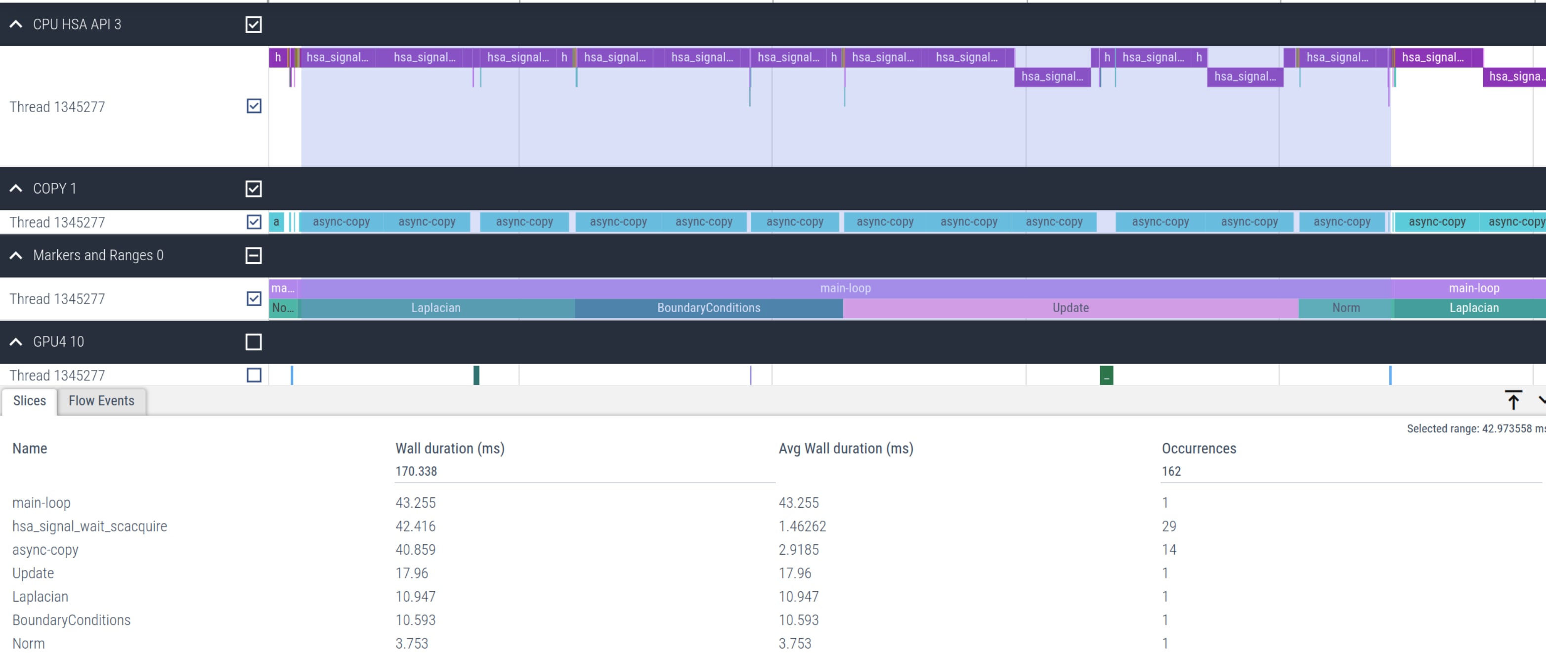
Figure 2: Timeline of Jacobi offload kernels using structured target data map

Unstructured Target Data Map

We note that most of the state variables that Jacobi solver requires can reside on the device. The data needs to be mapped to the host (CPU) only for the final residual output and the state solution data if required. Therefore, we can switch to unstructured target data mapping constructs which ensure data resides on the device between target enter data and target exit data map constructs. We perform the host to device copy before the Jacobi iterations and release the device data after the loops end, as shown below:

Copied!

void Jacobi_t::Run()
{
  const int N = mesh.N;
  #pragma omp target enter data map(to: mesh,h_U[0:N],h_AU[0:N],h_RES[0:N],h_RHS[0:N])

  ...
  while ((iterations < JACOBI_MAX_LOOPS) && (residual > JACOBI_TOLERANCE)) 
  {
    Laplacian(mesh, _1bydx2, _1bydy2, HD_U, HD_AU);
    BoundaryConditions(mesh, _1bydx2, _1bydy2, HD_U, HD_AU);
    Update(mesh, factor, HD_RHS, HD_AU, HD_RES, HD_U);
    residual = Norm(mesh, HD_RES);
    
    ++iterations;
  }
  ...

  #pragma omp target exit data map(release: h_U[0:N],h_AU[0:N],h_RES[0:N],h_RHS[0:N])
}

This avoids repetitive data mapping from host-to-device and device-to-host in every iteration that was needed by the structured target data map constructs for all the routines: Laplacian, BoundaryConditions, Update, and Norm. This essentially means removing the #pragma omp target data map() constructs in these routines.

For example, the code below shows now the updated Norm function has no structured map constructs in the target region any more. Here, the state vector $U$ is already mapped onto the device using the unstructured data map constructs at the very beginning of the Jacobi solver.

Copied!

dfloat Norm(mesh_t& mesh, dfloat *U) 
{
  dfloat norm = 0.0;
  const int N = mesh.N;
  const dfloat dx = mesh.dx;
  const dfloat dy = mesh.dy;
  #pragma omp target teams distribute parallel for reduction(+:norm)
  for (int id=0; id < N; id++) {
    norm += U[id] * U[id] * dx * dy;
  }
  return sqrt(norm)/N;
}

Figure 3 below shows the timeline of the major Jacobi solver kernels. The figure clearly shows that the total number of hsa_signal_wait_scacquire kernel calls are reduced by a significant amount compared to what was observed in the first naive offload implementation in Figure 2.

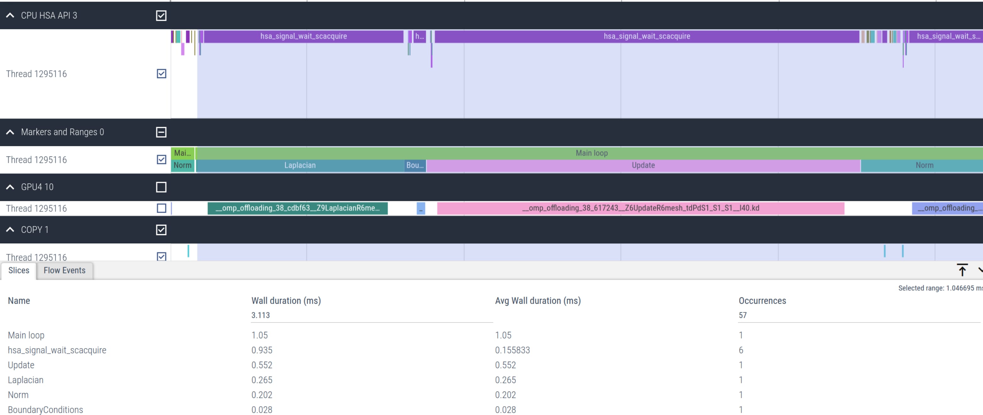
Figure 3: Timeline of the optimized Jacobi offload kernels using unstructured mapping

The following Table summarizes the timings of the main kernels of the Jacobi solver with OpenMP offload implementation using Clang compiler. The grid size is $4096 \times 4096$ , consistent with the HIP version. The total wall clock time over a thousand iterations is 999 ms[2] and is very comparable to the HIP implementation value observed earlier on one GCD of a MI250 GPU. A compute performance of 285 GFLOPs compares well with the value observed with the HIP implementation as well. Overall, the timings of the major code regions with the OpenMP offload are very close to the values obtained with HIP porting.

Kernels	Avg Time (ms)	Percentage
Update	0.51	57.9
Laplacian	0.25	27.6
Norm	0.11	12.2
BoundaryConditions	0.02	2.2

HIP vs OpenMP Offload

The Jacobi Solver with sparse matrix operations, whose Arithmetic Intensity (AI = FLOPs/Band Width) is about 0.17, lies in the memory bound regime. Therefore we compare the achieved memory Band Width (BW) of the kernels from HIP and OpenMP offload implementations. The following Table compares the HBM BW (GB/s) values from HIP and OpenMP offload implementations.

Kernels	HIP HBM BW (GB/s)	OpenMP Offload HBM BW (GB/s)
Update	1306	1297
Laplacian	1240	1091
Norm	1325	1239
BoundaryConditions	151	50

Most of the kernels achieve BW values very close to the achievable peak BW of MI250 of about [1300-1400] GB/s. The work done in BoundaryConditions is too small to saturate GPU, and therefore the values are small. Below in Figure 4 we show rooflines[3] from both HIP and OpenMP offload implementations of the Update kernel. As observed from the roofline figures, the Update kernel from both the implementations lie very close to the roofline in the memory bound regime. This agrees well with the observations made from the HBM table above.

Light Dark

Figure 4: Roofline of Update kernel using HIP (left) and OpenMP offload (right)

Similar observations about achieved BW for the Laplacian kernels are made from the rooflines below in Figure 5 from both the GPU offload implementations.

Light Dark

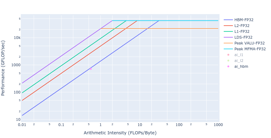
Figure 5: Roofline of Laplacian kernel using HIP (left) and OpenMP offload (right)

Conclusion

In this blog post, we have presented GPU offloading of a finite difference Jacobi Solver using HIP and OpenMP target offloading. The HIP implementation required replacing host codes with new HIP kernels, and optimizing on the kernel launch parameters including thread block and grid sizes as well as the launch bounds. On the other hand, the OpenMP offload implementation, being directive based, required less instrusive modifications to the existing host code base. For the problem sizes considered, the OpenMP offload could achieve compute performance and bandwidth metrics comparable, or even better at times, to the HIP GPU porting with significantly less coding effort. This illustrates the advantages that a directive based GPU porting such as OpenMP offload can offer compared to the approaches involving code rewrites such as HIP porting. Having said that, it is worth mentioning that for more complex applications, OpenMP may offer only limited options for tuning of the target offload constructs and its parameters for additional performance gains.

In the future, we will follow up this blog post with a Fortran OpenMP offload version of the Jacobi Solver.

Engines and APIs

Hybrid RT and samples

Our SDKs and libraries

Content creation

Blogs and videos

Performance guides

Reference

Latest news

Events

Research

Getting started with:

Jacobi Solver with HIP and OpenMP offloading

Jacobi Iterative Methods

Jacobi Code structure

Setup Jacobi Object

Execute Jacobi Method

GPU offload using HIP

GPU offload using OpenMP

Structured Target Data Map

Unstructured Target Data Map

HIP vs OpenMP Offload

Conclusion

Related content

Recent blog posts

Looking for a good place to get started with exploring GPUOpen?