Finite difference method – Laplacian part 2

Review

In the previous post, we considered a HIP implementation of the central finite difference stencil for the Laplacian. Recall that the Laplacian takes the form of a divergence of a gradient of a scalar field u(x,y,z):

\nabla \cdot \nabla u = \nabla^2 u = \frac{\partial^2u}{\partial x^2} + \frac{\partial^2u}{\partial y^2} + \frac{\partial^2u}{\partial z^2},

The initial HIP implementation is shown below

template <typename T>
__global__ void laplacian_kernel(T * f, const T * u, int nx, int ny, int nz, T invhx2, T invhy2, T invhz2, T invhxyz2) {

    int i = threadIdx.x + blockIdx.x * blockDim.x;
    int j = threadIdx.y + blockIdx.y * blockDim.y;
    int k = threadIdx.z + blockIdx.z * blockDim.z;

    // Exit if this thread is on the boundary
    if (i == 0 || i >= nx - 1 ||
        j == 0 || j >= ny - 1 ||
        k == 0 || k >= nz - 1)
        return;

    const int slice = nx * ny;
    size_t pos = i + nx * j + slice * k;
    
    // Compute the result of the stencil operation
    f[pos] = u[pos] * invhxyz2
           + (u[pos - 1]     + u[pos + 1]) * invhx2
           + (u[pos - nx]    + u[pos + nx]) * invhy2
           + (u[pos - slice] + u[pos + slice]) * invhz2;
} 

template <typename T>
void laplacian(T *d_f, T *d_u, int nx, int ny, int nz, int BLK_X, int BLK_Y, int BLK_Z, T hx, T hy, T hz) {

    dim3 block(BLK_X, BLK_Y, BLK_Z);
    dim3 grid((nx - 1) / block.x + 1, (ny - 1) / block.y + 1, (nz - 1) / block.z + 1);
    T invhx2 = (T)1./hx/hx;
    T invhy2 = (T)1./hy/hy;
    T invhz2 = (T)1./hz/hz;
    T invhxyz2 = -2. * (invhx2 + invhy2 + invhz2);

    laplacian_kernel<<<grid, block>>>(d_f, d_u, nx, ny, nz, invhx2, invhy2, invhz2, invhxyz2);
} 

and the corresponding performance on a single MI250X GCD:

$ ./laplacian_dp_kernel1 
Kernel: 1
Precision: double
nx,ny,nz = 512, 512, 512
block sizes = 256, 1, 1
Laplacian kernel took: 2.64172 ms, effective memory bandwidth: 808.148 GB/s 

The reported 808.148 GB/s meets 69.4% of the target we established in the previous post. We will continue to use rocprof to help us gauge the effectiveness of each of the following optimizations.

In the previous post, we can infer that the f device array is efficiently stored because the WRITE_SIZE metric matches the theoretical. However, the reported FETCH_SIZE is almost double the theoretical amount and therefore there can be an opportunity to improve performance if this data size could be reduced. Recall that seven elements from the u array are loaded to update each entry in the f array but each of those u elements could be reused up to six times by neighboring grid points. It is important to note that from a wavefront perspective, the load for each entry in u is a contiguous chunk of 64 entries. Our current thread block configuration (256 \times 1 \times 1) loads four waves of elements along the x direction, providing an opportunity for threads in a single wave to cache and reuse x elements for x - 1 and x + 1 stencil computations. However, loading waves in the y and z directions must be implemented carefully to maximize spatial locality and reuse values from neighboring waves and thread blocks. Thus, we focus our attention on optimizing loads in one of these two directions through loop tiling.

Loop tiling

As it stands, each thread computes a stencil around a single grid point. What happens if we let each thread compute stencils of multiple grid points? This will require more load instructions per thread but due to the contiguous nature of the threading, these loads will be more likely to reuse cached values for u. This optimization, known as loop tiling, will reduce the number of thread blocks launched and increase the number of stencils computed per thread.

Before we dive into the optimized Laplacian kernel, let us first consider a small example to further explain the concept and benefit of loop tiling: Suppose we want to perform the strided computation f[pos] = u[pos - 1] + u[pos] + u[pos + 1]. Without tiling, each thread would need to perform three loads and one store instruction. It would be ideal if we could have each thread only load one u element and reuse the other two u elements already loaded and stored in registers. In other words, we should try to minimize the number of loads per store instruction per thread. If we tile by some factor, let’s pick two, then each thread would perform two stores, but consider the number of loads:

f[pos]     = u[pos - 1]  + u[pos]     + u[pos + 1] 
f[pos + 1] = u[pos]      + u[pos + 1] + u[pos + 2]

Note that u[pos] and u[pos + 1] appear twice, which means we only need to load them once. This observation allows us to reuse the previously loaded value. To make this point clear, we can introduce two variables:

double u0 = u[pos];
double u1 = u[pos + 1]
f[pos]     = u[pos - 1] + u0  + u1
f[pos + 1] = u0         + u1  + u[pos + 2]

As a result, we have explicitly reduced the number of load instructions from 6 to 4 (i.e., reduction by 33%). We now have approximately 2 loads per store. See the table below to see how loop tiling factors correlate with the load store ratio.

Keep in mind that the increasing the tile factor increases the register use in the kernel which will reduce its occupancy. If the compiler runs out of registers, register spillage to global memory occurs which can negatively affect performance.

Circling back to the 3D Laplacian kernel, there are three potential directions for loop tiling. Let us tile in the y-direction for demonstration. Consider the figure below illustrating the reuse pattern:

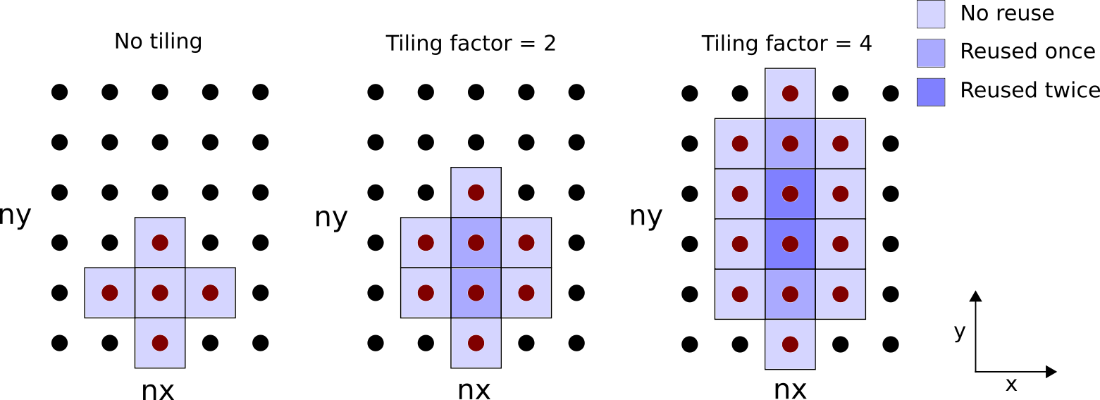
Figure 1: Illustration of loop tiling for each thread on an xy plane. The number of grid points loaded and reused depends on the tile width.

Let us denote the tile factor by m, which is a user defined macro variable determined at compile time. The code modifications for this kernel can be quite complex so we shall cover the changes in two phases: setup and computation. First, we apply the following changes:

 



int j = threadIdx.y + blockIdx.y * blockDim.y;

...

// Exit if this thread is on the boundary
if (i == 0 || i >= nx - 1 ||
    j == 0 || j >= ny - 1 ||
    k == 0 || k >= nz - 1)
    return;

...

dim3 grid((nx - 1) / block.x + 1, 
          (ny - 1) / block.y + 1, 
          (nz - 1) / block.z + 1);

#define m 1

...

int j = m*(threadIdx.y + blockIdx.y * blockDim.y);

...

// Exit if this thread is on the xz boundary
if (i == 0 || i >= nx - 1 ||
    k == 0 || k >= nz - 1)
    return;

...
 
 
dim3 grid((nx - 1) / block.x + 1, 
          (ny - 1) / (block.y * m) + 1, 
          (nz - 1) / block.z + 1);

Kernel 2 introduces the macro variable m which is used to divide the grid dimension in the y direction. Setting m=1 currently has no tiling effect – experimenting with other values requires recompilation of the code. We removed the requirement that threads exit at the y boundary for the case where stencils overlap the boundary.

In our next set of code modifications, we focus on rewriting the f[pos] = ... computation for a tile factor m. Because we are tiling in the y direction, each thread strides pos by nx. These modifications are tricky so we will break it down into four steps:

1. Add a for loop to the main computational kernel

2. Introduce an array of size m to accumulate the running sum of the stencil points

3. Split the u element loads and f element stores into separate loops

4. Introduce a variable to hold a u element for reuse

Below are code snippets before and after the application of the four steps. We begin by wrapping our stencil evaluation in a for loop:

 
 
f[pos] = u[pos] * invhxyz2
       + (u[pos - 1]     + u[pos + 1]) * invhx2
       + (u[pos - nx]    + u[pos + nx]) * invhy2
       + (u[pos - slice] + u[pos + slice]) * invhz2;

for (int n = 0; n < m; n++)
  if (j + n > 0 && j + n < ny - 1)
    f[pos + n*nx] = u[pos + n*nx] * invhxyz2
       + (u[pos - 1 + n*nx]     + u[pos + 1 + n*nx]) * invhx2
       + (u[pos - nx + n*nx]    + u[pos + nx + n*nx]) * invhy2
       + (u[pos - slice + n*nx] + u[pos + slice + n*nx]) * invhz2;

Introducing a for loop over a value m known at compile time has similar effects to loop unrolling where the compiler will minimize the overhead of looping. Keep in mind m must not be too large or the compiler will spill registers to global memory.

At this point, the kernel is technically tiled, however, a few more code modifications are needed to minimize the load to store ratio. Next we create an accumulation array:

 
for (int n = 0; n < m; n++)
  if (j + n > 0 && j + n < ny - 1)
    f[pos + n*nx] = u[pos + n*nx] * invhxyz2
       + (u[pos - 1 + n*nx]     + u[pos + 1 + n*nx]) * invhx2
       + (u[pos - nx + n*nx]    + u[pos + nx + n*nx]) * invhy2
       + (u[pos - slice + n*nx] + u[pos + slice + n*nx]) * invhz2;
 
 

T Lu[m] = {0};
for (int n = 0; n < m; n++)
  if (j + n > 0 && j + n < ny - 1) {
    Lu[n] = u[pos + n*nx] * invhxyz2;
    Lu[n] += (u[pos - 1 + n*nx]     + u[pos + 1 + n*nx]) * invhx2;
    Lu[n] += (u[pos - nx + n*nx]    + u[pos + nx + n*nx]) * invhy2;
    Lu[n] += (u[pos - slice + n*nx] + u[pos + slice + n*nx]) * invhz2;
    f[pos + n*nx] = Lu[n];
  }

The accumulation array Lu temporarily holds the sum of the computations. Note that we kept the original order of the stencil computations – first load the x direction stencils, then the y direction stencils, and finally the z direction stencils. We will eventually revisit this ordering, but our next step is to split the load and store steps:

T Lu[m] = {0};
for (int n = 0; n < m; n++)
  if (j + n > 0 && j + n < ny - 1) {
    Lu[n] = u[pos + n*nx] * invhxyz2;
    Lu[n] += (u[pos - 1 + n*nx]     + u[pos + 1 + n*nx]) * invhx2;
    Lu[n] += (u[pos - nx + n*nx]    + u[pos + nx + n*nx]) * invhy2;
    Lu[n] += (u[pos - slice + n*nx] + u[pos + slice + n*nx]) * invhz2;
    f[pos + n*nx] = Lu[n];
  }
  
 

T Lu[m] = {0};
for (int n = 0; n < m; n++)
  if (j + n > 0 && j + n < ny - 1) {
    Lu[n] = u[pos + n*nx] * invhxyz2;
    Lu[n] += (u[pos - 1 + n*nx]     + u[pos + 1 + n*nx]) * invhx2;
    Lu[n] += (u[pos - nx + n*nx]    + u[pos + nx + n*nx]) * invhy2;
    Lu[n] += (u[pos - slice + n*nx] + u[pos + slice + n*nx]) * invhz2;
  }
for (int n = 0; n < m; n++)
  if (j + n > 0 && j + n < ny - 1)
    f[pos + n*nx] = Lu[n];

Splitting the loads and stores into separate for loops enables all Lu elements to simultaneously accumulate the stencil computations before writing to f. The fourth and final change is to explicitly remove load instructions by reusing loaded u elements across different stencils. Each iteration of n still loads the x direction and z direction stencils for Lu[n] but could now potentially reuse the u element to compute y direction stencils belonging to Lu[n-1] and/or Lu[n+1]:

 
T Lu[m] = {0};
for (int n = 0; n < m; n++)
  if (j + n > 0 && j + n < ny - 1) {
    Lu[n] = u[pos + n*nx] * invhxyz2;
    Lu[n] += (u[pos - 1 + n*nx]     + u[pos + 1 + n*nx]) * invhx2;
    Lu[n] += (u[pos - nx + n*nx]    + u[pos + nx + n*nx]) * invhy2;
    Lu[n] += (u[pos - slice + n*nx] + u[pos + slice + n*nx]) * invhz2;
  }
for (int n = 0; n < m; n++)
  if (j + n > 0 && j + n < ny - 1)
    f[pos + n*nx] = Lu[n];
  
 
 

T center;
T Lu[m] = {0};
for (int n = 0; n < m; n++) {
  center = u[pos + n*nx];
  Lu[n] = center * invhxyz2 
        + (u[pos - 1 + n*nx]     + u[pos + 1 + n*nx]) * invhx2;
  if (n == 0) Lu[n] += u[pos - nx + n*nx] * invhy2;
  if (n > 0) Lu[n-1] += center * invhy2;
  if (n < m - 1) Lu[n+1] += center * invhy2;
  if (n == m - 1) Lu[n] += u[pos + nx + n*nx] * invhy2;
  Lu[n] += (u[pos - slice + n*nx] + u[pos + slice + n*nx]) * invhz2;
}
for (int n = 0; n < m; n++)
  if (j + n > 0 && j + n < ny - 1)
    f[pos + n*nx] = Lu[n];

Below is the full kernel 2 implementation capturing all the above code modifications:

// Tiling factor
#define m 1
template <typename T>
__global__ void laplacian_kernel(T * f, const T * u, int nx, int ny, int nz, T invhx2, T invhy2, T invhz2, T invhxyz2) {
    
    int i = threadIdx.x + blockIdx.x * blockDim.x;
    int j = m*(threadIdx.y + blockIdx.y * blockDim.y);
    int k = threadIdx.z + blockIdx.z * blockDim.z;
    
    // Exit if this thread is on the xz boundary
    if (i == 0 || i >= nx - 1 ||
        k == 0 || k >= nz - 1)
        return;
    
    const int slice = nx * ny;
    size_t pos = i + nx * j + slice * k;

    // Each thread accumulates m stencils in the y direction
    T Lu[m] = {0};

    // Scalar for reusable data
    T center;

    // Loop tiling
    for (int n = 0; n < m; n++) {
        center = u[pos + n*nx]; // store for reuse
  
        // x direction
        Lu[n] += center *invhxyz2
              + (u[pos - 1 + n*nx] + u[pos + 1 + n*nx]) * invhx2;
  
        // y - 1, first n
        if (n == 0) Lu[n] += u[pos - nx + n*nx] * invhy2;
  
        // reuse: y + 1 for prev n
        if (n > 0) Lu[n-1] += center * invhy2;
  
        // reuse: y - 1 for next n
        if (n < m - 1) Lu[n+1] += center * invhy2;
  
        // y + 1, last n
        if (n == m - 1) Lu[n] += u[pos + nx + n*nx] * invhy2;
  
        // z - 1 and z + 1
        Lu[n] += (u[pos - slice + n*nx] + u[pos + slice + n*nx]) * invhz2;
    }

    // Store only if thread is inside y boundary
    for (int n = 0; n < m; n++)
      if (j + n > 0 && j + n < ny - 1)
        f[pos + n*nx] = Lu[n];
 }

template <typename T>
void laplacian(T *d_f, T *d_u, int nx, int ny, int nz, int BLK_X, int BLK_Y, int BLK_Z, T hx, T hy, T hz) {

    dim3 block(BLK_X, BLK_Y, BLK_Z);
    dim3 grid((nx - 1) / block.x + 1, (ny - 1) / (block.y * m) + 1, (nz - 1) / block.z + 1);
    T invhx2 = (T)1./hx/hx;
    T invhy2 = (T)1./hy/hy;
    T invhz2 = (T)1./hz/hz;
    T invhxyz2 = -2. * (invhx2 + invhy2 + invhz2);

    laplacian_kernel<<<grid, block>>>(d_f, d_u, nx, ny, nz, invhx2, invhy2, invhz2, invhxyz2);
} 

Note that this kernel is currently written so that ny must be divisible by block.y * m. Let us experiment with various values of m compatible with our chosen problem size and see whether loop tiling has any benefits.

It is strange that none of the examined m provide any significant speedup. In fact, increasing the tile factor appears to exacerbate the performance. Let’s examine the FETCH_SIZE and L2CacheHit metrics for further insight:

The fetch efficiency only marginally increased whereas the L2 cache hit drops significantly. We suspect the reason for this is that the accumulation steps follow the same access pattern as the initial kernel. That is, we first compute the x direction stencils, followed by the potentially reusable y - 1 and y + 1 stencils, and end with the z - 1 and z + 1 stencils. From a memory address perspective, the read access pattern jumps both forward and backward which could have implications, as explained and addressed next.

Reorder read access patterns

After the optimization, there is little to no speedup. While increasing the tile factor reduces the loads per store ratio, it may not necessarily translate into a reduction in global data movement. For FETCH_SIZE to decrease, the data movement between L2 and global memory must decrease. As the load per store ratio increases, the number of read requests sent to L1 must decrease and L2 as well (assuming that the L1 cache hit ratio stays the same). Since we observe that FETCH_SIZE stays the same and that L2CacheHit decreases, the optimization has reduced the pressure on the L2 cache (fewer requests sent to it) but failed to improve the reuse of the data loaded from global memory into the L2 cache. To understand why the previous kernel achieves suboptimal L2 data reuse, let us visualize the 3D stencils and their read access patterns if m = 2:

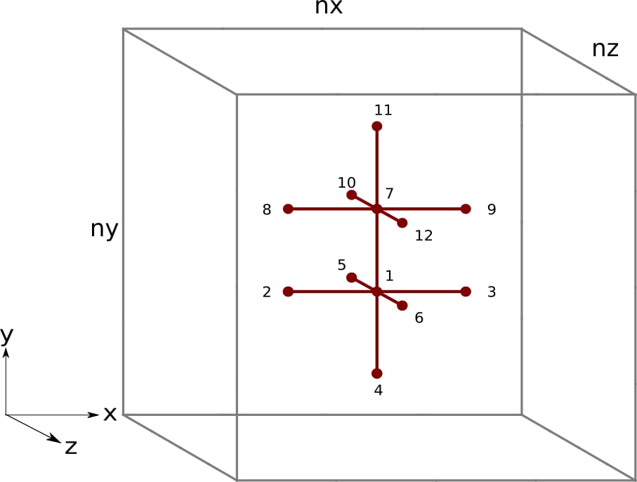
Figure 2: Finite difference stencil in 3D space with a tile factor of m = 2. The black numbers represent the order each thread in Kernel 2 accesses elements of u.

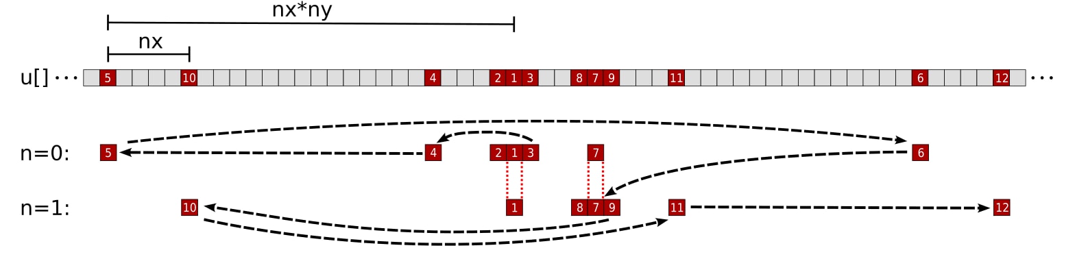
Figure 3: Kernel 2 memory access pattern of a single thread for the array u with a tile factor of m = 2. The numbers and black arrows correspond to the order the thread accesses elements of u. The n = 0 and n = 1 rows represent u elements needed for the stencil computation of grid points pos and pos + nx, respectively. The 1st accessed element (u[pos]) is loaded during the n = 0 iteration and reused for the y - 1 element of the n = 1 iteration. Likewise the 7th accessed element (u[pos + nx]) is loaded during the n = 1 iteration and reused for the y + 1 element of the n = 0 iteration.

We immediately see a problem. The thread often needs to jump “backwards” in the memory space of the u array. After accessing each grid point’s z + 1 element, the thread needs to jump “backwards” to access the x direction elements for the next iteration of n. Frequently accessing u elements by going both forward and backward in the memory address may prematurely evict reusable data from cache. We prefer to instead reorder the instructions in the kernel to only use a single direction i.e., accessing memory by ascending address:

Figure 4: Finite difference stencil in 3D space with a tile factor of m = 2. The black numbers represent the order each thread the proposed kernel accesses elements of u.

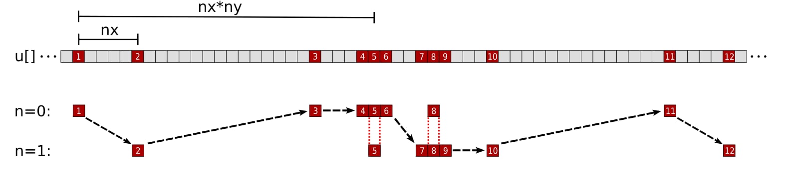
Figure 5: Proposed memory access pattern of a single thread for the array u with a tile factor of m = 2. The numbers and black arrows correspond to the order the thread accesses elements of u. The n = 0 and n = 1 rows represent u elements needed for the stencil computation of grid points pos and pos + nx, respectively. The 5th accessed element (u[pos]) is loaded during the n = 0 iteration and reused for the y - 1 element of the n = 1 iteration. Likewise the 8th accessed element (u[pos + nx]) is loaded during the n = 1 iteration and reused for the y + 1 element of the n = 0 iteration.

Under this different approach, we first access all z - 1 elements, followed by the y - 1 element of iteration n = 0, all x direction elements, the y + 1 element of iteration n = m - 1, and end with all z + 1 elements. Each thread now accesses all needed u elements by ascending memory address. A significant rewrite of the kernel is necessary, so we first present the full implementation:

// Tiling factor
#define m 1
template <typename T>
__global__ void laplacian_kernel(T * f, const T * u, int nx, int ny, int nz, T invhx2, T invhy2, T invhz2, T invhxyz2) {
    
    int i = threadIdx.x + blockIdx.x * blockDim.x;
    int j = m*(threadIdx.y + blockIdx.y * blockDim.y);
    int k = threadIdx.z + blockIdx.z * blockDim.z;
    
    // Exit if this thread is on the xz boundary
    if (i == 0 || i >= nx - 1 ||
        k == 0 || k >= nz - 1)
        return;
    
    const int slice = nx * ny;
    size_t pos = i + nx * j + slice * k;
    
    // Each thread accumulates m stencils in the y direction
    T Lu[m] = {0};
    
    // Scalar for reusable data
    T center;
    
    // z - 1, loop tiling
    for (int n = 0; n < m; n++)
        Lu[n] += u[pos - slice + n*nx] * invhz2;
    
    // y - 1
    Lu[0]   += j > 0 ? u[pos - 1*nx] * invhy2 : 0; // bound check
    
    // x direction, loop tiling
    for (int n = 0; n < m; n++) {
        // x - 1
        Lu[n] += u[pos - 1 + n*nx] * invhx2;

        // x
        center = u[pos + n*nx]; // store for reuse
        Lu[n] += center * invhxyz2;

        // x + 1
        Lu[n] += u[pos + 1 + n*nx] * invhx2;
        
        // reuse: y + 1 for prev n
        if (n > 0) Lu[n-1] += center * invhy2;

        // reuse: y - 1 for next n
        if (n < m - 1) Lu[n+1] += center * invhy2;
    }
    
    // y + 1
    Lu[m-1]  += j < ny - m ? u[pos + m*nx] * invhy2 : 0; // bound check
    
    // z + 1, loop tiling
    for (int n = 0; n < m; n++)
      Lu[n] += u[pos + slice + n*nx] * invhz2;

    // Store only if thread is inside y boundary
    for (int n = 0; n < m; n++)
      if (n + j > 0 && n + j < ny - 1)
        f[pos + n*nx] = Lu[n];
} 

template <typename T>
void laplacian(T *d_f, T *d_u, int nx, int ny, int nz, int BLK_X, int BLK_Y, int BLK_Z, T hx, T hy, T hz) {

    dim3 block(BLK_X, BLK_Y, BLK_Z);
    dim3 grid((nx - 1) / block.x + 1, (ny - 1) / (block.y * m) + 1, (nz - 1) / block.z + 1);
    T invhx2 = (T)1./hx/hx;
    T invhy2 = (T)1./hy/hy;
    T invhz2 = (T)1./hz/hz;
    T invhxyz2 = -2. * (invhx2 + invhy2 + invhz2);

    laplacian_kernel<<<grid, block>>>(d_f, d_u, nx, ny, nz, invhx2, invhy2, invhz2, invhxyz2);
} 

We now go into the details of the computational steps within this kernel. First, we access all z - 1 grid points followed by a single y - 1:

    // z - 1, loop tiling
    for (int n = 0; n < m; n++)
        Lu[n] += u[pos - slice + n*nx] * invhz2;
    
    // y - 1
    Lu[0]   += j > 0 ? u[pos - 1*nx] * invhy2 : 0; // bound check

Note that the conditional operator is introduced so that it computes the y - 1 stencil for the n = 0 grid point only if it does not lie on the y boundary. Neither the z - 1 nor y - 1 elements are reused at the thread level.

Next, the thread computes the xdirection stencils:

    // x direction, loop tiling
    for (int n = 0; n < m; n++) {
        // x - 1
        Lu[n] += u[pos - 1 + n*nx] * invhx2;

        // x
        center = u[pos + n*nx]; // store for reuse
        Lu[n] += center * invhxyz2;

        // x + 1
        Lu[n] += u[pos + 1 + n*nx] * invhx2;
        
        // reuse: y + 1 for prev n
        if (n > 0) Lu[n-1] += center * invhy2;

        // reuse: y - 1 for next n
        if (n < m - 1) Lu[n+1] += center * invhy2;
    }

Again, neither the x - 1 nor x + 1 points are reused at the thread level, but the center element u[pos + n*nx] could be reused up to two times as in the previous kernel.

Afterwards, we load the final y + 1 point as well as all the z + 1 points:

    // y + 1
    Lu[m-1]  += j < ny - m ? u[pos + m*nx] * invhy2 : 0; // bound check
    
    // z + 1, loop tiling
    for (int n = 0; n < m; n++)
      Lu[n] += u[pos + slice + n*nx] * invhz2;

Another conditional operator is used so that it computes the y + 1 stencil of the n = m - 1 grid point so long as it does not lie on the y boundary.

Lastly, all threads inside the y boundary are written back to memory:

    // Store only if thread is inside y boundary
    for (int n = 0; n < m; n++)
      if (n + j > 0 && n + j < ny - 1)
        f[pos + n*nx] = Lu[n];

Let us now experiment with the same tile factors and see if this reordering makes any difference:

Even if m=1, the reordered access pattern for u elements already provides a significant boost in performance. The incremental improvements in speedup for each m is what we were expecting to see. Let us examine the rocprof metrics for this new kernel:

The FETCH_SIZE metric decreased significant, bringing us remarkably close to the theoretical limit. The L2CacheHit rate not only increased but now exceeds what we were originally getting from the baseline kernel. However, we note that there is a significant drop in the cache hit rate coupled with a significant increase in the fetch sizes when m=16. For the chosen problem, kernel 3 with m=8 is our best kernel yet, achieving almost 95% of the target effective memory bandwidth and over 99% fetch efficiency.

Summary

With both optimizations combined, the FETCH_SIZE is reduced by up to 2x. This suggests that our HIP kernel can load data efficiently for a specific grid size. To accomplish this, we first reduced the number of loads per store instruction by explicitly evaluating multiple stencils via loop tiling. However, our initial implementation did not improve performance. To address this, we reordered the memory access pattern to improve the L2 cache hit ratio. The question now is whether we are “done” optimizing our initial HIP implementation of the finite difference method for the Laplacian. We must address a few lingering issues first:

1. Is there room for further performance improvement? We have already optimized the memory movement between L2 cache and global memory, so we must look at other areas for performance gains e.g., latency hiding.

2. Why does the performance of m=16 degrade significantly? This happens with or without the reordering of memory access. Perhaps resolving the underlying issues may help us get closer to the target?

3. How do other architectures and problem sizes impact the choice of tile factors? All of our optimizations thus far are tailored towards a single MI250X GCD on a problem size of nx,ny,nz = 512, 512, 512.

The next post in this series will answer some of these remaining open questions.

Accompanying code examples

If you have any questions or comments, please reach out to us on GitHub Discussions