CPU performance optimization guide – part 3

1.1. Instruction selection

First of all, the latency of each instruction in the CPU is not the same. We choose the most common integer instruction this time, and the goal is to get the nearest square root of the integer using only the integer instruction.

1.2. Compiler

Then comes the compiler. Due to the popularity and ease of use of Microsoft Windows® 10, Microsoft Visual Studio® 2022 is selected as the development environment, version 17.9.2. The compiler version is 19.39.33521. The compiler type is x64 RelWithDebInfo. The operating system version is 10.0.19045.4046.

1.3. CPU and performance analyzer

Finally, the CPU needs to be identified because the architecture is constantly being updated. The latency of each instruction varies from CPU to CPU. And because of the strong dependence on hardware, the CPU determines the performance analyzer can be used. The CPU used here is an AMD Ryzen™ 9 7900X3D, so the performance analyzer used here is AMD μProf, version 4.2.845.

2.1. Data preparation

As the goal is relatively simple this time, our data set is all the unsigned integer ranges that uint32_t can cover, which is of sufficient magnitude to ensure the accuracy of the performance data.

The algorithm needs to be verified. Each integer will be compared with the result of std::sqrt to ensure the correctness of the algorithm.

2.2. Test function

The test function is the focus of this blog. When it comes to the challenge of using only integer instructions to get the nearest square root of an integer, the simplest and fastest design I have encountered is Microchip TB040. It makes use of the bit operation of integers, which makes the calculation amount of the algorithm tend to be linear. The following is a simple implementation. For exactly how it works, you can refer to the paper itself.

1. uint32_t TB040(uint32_t x) {
2.     uint64_t x_ = x;
3.     uint32_t res = 0;
4.     uint32_t add = 0x80000000;
5. 
6.     while (add) {
7.         uint32_t g = res | add;
8.         if (x_ >= (static_cast<uint64_t>(g) * g)) {
9.             res = g;
10.         }
11.         add >>= 1;
12.     }
13.     return res;
14. }

TB040 is quite good already, especially on the hardware-limited single-chip microcomputer. But it can still be improved. When the algorithm itself is already good enough, reducing its workload is a good direction to optimize. On hardware with good bit calculation support, the add variable in TB040 may not be initialized to a fixed value but may be set according to the position of the most significant bit of x. Due to the nature of the square root, the initial position of add can be set to half the index of the most significant bit of x to reduce the amount of computation.

15. inline unsigned long clzll(uint32_t v) {
16.     unsigned long lz = 0;
17.     _BitScanReverse(&lz, v);
18.     return lz;
19. }
20. 
21. uint32_t add = 1 << (clzll(x) >> 1);

Here we use the bsr instruction to fetch the most significant bit. Instructions such as lzcnt and std::bit_width() in C++20 have similar functionality, but we’ll leave it to the readers to explore.

2.3. Performance data

The performance test needs to be run a few more times and average the data to prevent hopping. It is clear that the optimized TB040 runs faster than the original TB040. The data is as expected, because the displacement reduces the amount of computation by at least half, which allows the algorithm to achieve greater throughput.

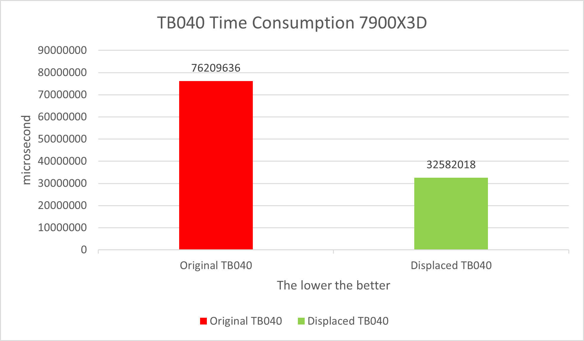
Table 1

3.1. Analyze PMC

Use the Performance Analyzer to analyze PMC, using Assess Performance (Extended) for the option set. After the run, switch to the ANALYZE page, and then switch to the IPC view to check the instructions and the PMCs. The CPU clock running is CYCLES_NOT_IN_HALT, and the number of instructions is RETIRED_INST.

Dividing RETIRED_INST by CYCLES_NOT_IN_HALT gives us the IPC, which is the number of instructions run per unit of time. The higher the IPC, the better. Do it in reverse gives us the CPI, which is the CPU clock consumed by a single instruction. The lower the CPI, the better. These names may vary in different versions of the performance analyzer. It hinges on the corresponding hardware PMC in the PPR.

3.2. TB040

Let’s start with the data of the original TB040. IPC performs well with few problems. Let’s keep in mind the CPU clock and the number of instructions.

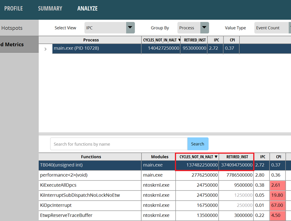
Figure 1: the original TB040

3.3. The displaced TB040

Let’s look at the data of the displaced TB040. IPC performs better, with less than half the CPU clock and about half the number of instructions compared to the original TB040. Obviously, if we want to optimize an algorithm that is already pleasing enough, a feasible way is to minimize the number of instructions and the CPU clock.

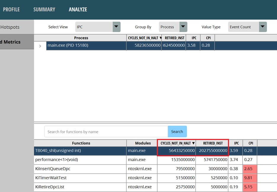
Figure 2: the displaced TB404