AMD FidelityFX™ Parallel Sort
AMD FidelityFX Parallel Sort makes sorting data on the GPU quicker, and easier. Use our SM6.0 compute shaders to get your data in order.
The primary goal of this article is to consolidate knowledge on transformations in Computer Graphics into a single, comprehensive resource.
Although these concepts are widely available online, they are often presented in disconnected fragments, lacking cohesive explanations of their subtleties. This article seeks to address those gaps and provide a thorough understanding of the topic.
Many real-world problems initially appear simple, but their underlying complexity becomes evident upon closer examination. To explore these challenges comprehensively, we will employ the well-known divide and conquer technique. By breaking this intricate problem into smaller sub-problems and addressing each individually, we can create a structured reference guide.
This approach will bring clarity and organization to the challenges often encountered in transformations within computer graphics.
These sub-problems can be categorized from both a mathematical (theoretical) and an implementation (practical) perspective as follows:
The order of matrix multiplication: Ensuring operations follow consistent sequencing rules.
The handedness of three-dimensional Euclidean space: Determining orientation conventions, such as the right-hand rule.
The order of basis vectors in a Cartesian coordinate system: Establishing the sequence for defining axes.
The storage of matrices in memory as multidimensional arrays: Optimizing memory representation for efficient computations.
In this article, we will explore matrices and their properties in depth. Before diving into the details, let’s briefly cover a few foundational concepts that are essential for understanding their nuances.
In mathematics, a matrix is essentially a rectangular array of numbers organized into rows and columns.
For example, the matrix below has 3 rows and 5 columns and can be referred to as a matrix:
The answer can be summarized by the following points:
They serve as an excellent algebraic tool for representing geometry in a structured way.
Transformations such as Affine and Projective in three-dimensional Euclidean space can be represented using matrices.
Concatenation of transformations, or combining two transformations, can be expressed as matrix multiplication.
Matrices with one row or column (in other words, row or column vectors) can store mesh vertices.
Transformation of mesh vertices from one space to another is, once again, a usage of matrix multiplication.
Matrices themselves and operations on them can be efficiently implemented in computer graphics applications.
The algorithm for matrix multiplication is not as straightforward as matrix addition, where corresponding elements from both matrices are added component-wise. Instead, it is slightly more complex and involves combining rows and columns through a series of operations.
To illustrate this concept, consider the following visualization:
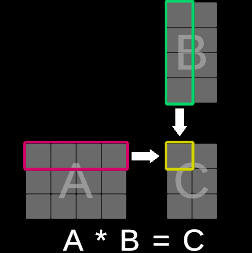
The value of each element in matrix C is calculated by multiplying each corresponding entry in the iᵗʰ row of matrix A with the jᵗʰ column of matrix B and summing these products. In essence, this operation is equivalent to performing a dot product between the iᵗʰ row of matrix A and the jᵗʰ column of matrix B.
It is important to note:
Matrix multiplication is generally not commutative—the order of multiplicands in multiplication matters.
For matrix multiplication to be valid, the number of columns in the first matrix (on the left side of the operator) must match the number of rows in the second matrix.
Once we have completed the preliminary explanations, we can shift our attention to the core of this article.
Now that we understand matrix multiplication, we can discuss its order. One of the key—yet often overlooked—aspects of transformations in computer graphics is that matrix multiplication is generally non-commutative.
We are accustomed to the fact that multiplication of real numbers is commutative. Therefore, when we learn about matrices, it is surprising—and often leads to errors in practice—that matrix multiplication is non-commutative:
where and are matrices.
To minimize challenges in practice, two distinct approaches—or conventions—have emerged, each offering a method for ensuring consistent and correct application of matrix multiplication.
In computer graphics, these conventions are referred to as:
Pre-multiplication Transformation
Post-multiplication Transformation
It is worth noting that the terminology of pre- and post-multiplication is used by some authors but not universally.
For example, in linear algebra, vectors are typically treated as column vectors when solving systems of equations, leading to a preference for post-multiplication order in textbooks.
In computer graphics applications, transformations such as translation, rotation, scaling, and shearing are combined to create realistic virtual worlds. These transformations are represented using matrices, and combining them is equivalent to multiplying matrices.
It is crucial to choose and apply the correct order consistently to achieve the desired result.
While matrix multiplication is non-commutative, it remains associative:
In the examples below, parentheses are used solely to indicate the order in which transformations are combined.
Let’s describe the problem of matrix multiplication order for transformation concatenation using the following example:
where , , , , are matrices.
Parentheses are helpful to clearly indicate the sequence (order) of operations. In mathematics, multiplication is typically assumed to proceed from left to right.
The differences between the two conventions are summarized in the table below:
| Post-multiplication | Pre-multiplication | |
|---|---|---|
| Order of operations | ||
| Transforming a vector | ||
| Vector representation | ||
| Final Transformation Matrix | ||
| World Matrix Composition | ||
| Local Transformation Matrix | ||
| Local Transformation Matrix | ||
| Impact of convention | Transformations composed right-to-left | Transformations composed left-to-right |
| Impact of convention | Preferred matrix storage in column-major layout | Preferred matrix storage in row-major layout |
| Impact of convention | Mesh vertices treated as column vectors | Mesh vertices treated as row vectors |
Where:
= Transformed vector in another space.
= Transformed vector in original space.
= Transform matrix.
= Final transformation matrix.
= Model transformation matrix (transforms from local model space to global world space).
= View matrix (transforms from world space to camera space).
= Projection matrix (transforms from camera space to clipping space).
= World transformation matrix.
= Current local transformation matrix.
= Transformation matrix of the parent node.
= Scaling matrix.
= Rotation matrix.
= Translation matrix.
= Shear matrix.
Before discussing the topic of the orientation of three-dimensional Euclidean space, one more issue should be mentioned and described: the “Up Direction” axial convention.
Mathematically, no axis is inherently designated as the Up Direction in three-dimensional Euclidean space.
However, in 3D applications, two conventions have emerged over the years:
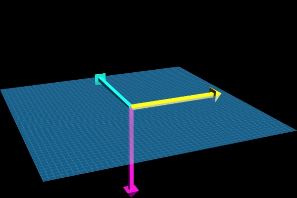
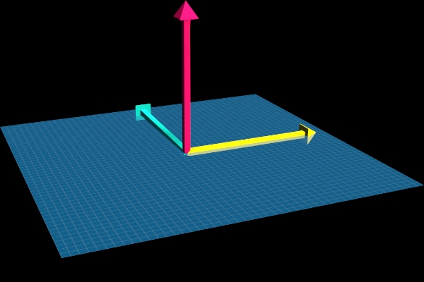
-Axis as “Up Direction”
This convention is particularly useful in fields such as architecture. When the working space is a plane representing, for example, the Earth’s surface, the two main working directions are the -Axis and -Axis, while the -Axis represents elevation, or the “Up Direction.”
-Axis as “Up Direction”
In this convention, the working plane corresponds to the monitor screen. The -Axis and -Axis represent the width and height of the screen, respectively, while the -Axis represents depth. This setup aligns with our everyday perception of the world, such as in first-person shooter (FPS) games, where the -Axis represents the “Up Direction.”
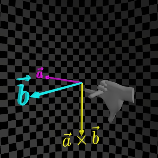
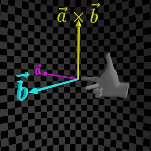
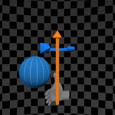
In computer graphics, particularly in three-dimensional Euclidean space, the cross product is a highly useful and common operation. The cross product of two non-collinear vectors results in another vector that is perpendicular to both original vectors.
This operation introduces ambiguity because the direction of the resulting vector does not have a unique solution—it could point in two equally valid directions. To resolve this ambiguity, we select an orientation (or handedness) for the three-dimensional Euclidean space. By making this choice, we designate one cross-product direction as the preferred solution.

To get a unique and consistent result, we use either the right-hand rule or the left-hand rule.
It is worth mentioning that in mathematics and physics, the right-hand orientation is the most commonly used. This orientation is applied to determine directions in magnetic fields, electromagnetic fields, and enantiomers in chemistry.
| Left-Hand Rule | Right-Hand Rule |
|---|---|
 |  |
The right-hand rule and left-hand rule can be described as follows:
Let the straightened index finger of the chosen hand (right or left) point in the direction of the first vector (), and let the bent middle finger point in the direction of the second vector (). Finally, the extended thumb will indicate the direction of the cross-product vector .
To determine the directions of the , , and axes in three-dimensional Euclidean space, replace the first vector with the direction of the -Axis and the second vector with the direction of the -Axis. The thumb will then indicate the direction of the -Axis.
Using this method, we can designate a three-dimensional Euclidean space with the desired handedness (orientation). The orientations, right-hand or left-hand, can be summarized in the table below (if applicable).
| Handedness | Left-Hand Rule | Right-Hand Rule |
|---|---|---|
| Y-Up | 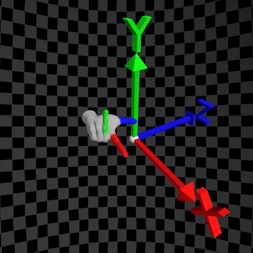 | 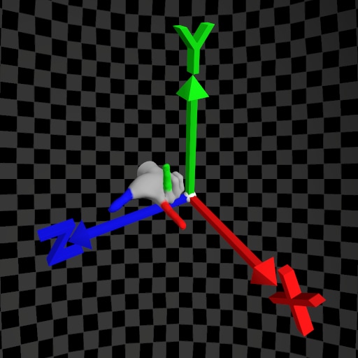 |
| Z-Up | 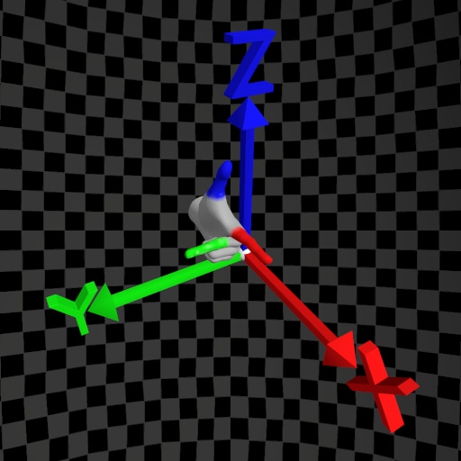 | 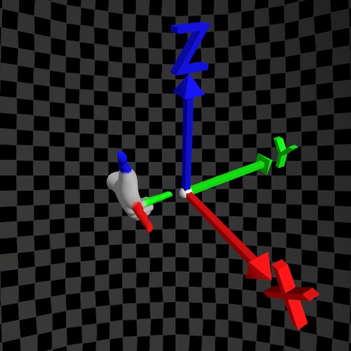 |
Choosing the handedness is crucial as it determines not only the direction of the cross-product vector but also:
The orientation of surface normal vectors.
The direction in which points rotate around an axis.
The order of vertices in triangle meshes.
| Left-Hand Rule | Right-Hand Rule |
|---|---|
 |  |
 |  |
Another key property of the cross product of two non-collinear vectors is anticommutativity:
If you need to fix a rendering error by reversing the result of a cross product, keep in mind that you are not simply adding a *negative sign* to the vector. Instead, you are altering the handedness of your three-dimensional Euclidean space.
| Left-Hand Rule | Right-Hand Rule |
|---|---|
 |  |
This topic should be introduced prior to the concept of handedness in Euclidean space, as the two are closely related. It is usually covered earlier in linear algebra classes. However, describing it now will make it easier to understand.
The concept of basis vectors often remains hidden in the shadows of linear algebra textbooks, and its significance is frequently overlooked, despite being fundamental to linear algebra and vector spaces.
For example, in three-dimensional Euclidean space, the following basis vectors:
form the building blocks of the Euclidean space. They allow any vector in this space to be described in terms of these basis vectors.
However, defining the basis vectors is only part of the process—it is also necessary to determine their order, specifying which vector is designated as the first, second, and third. For example:
 |  |
The order of the basis vectors is important because, while coordinate systems defined by different orders may appear similar, they are not the same and differ in subtle ways:
When the basis vectors and their order are determined, we establish the Cartesian coordinate system. This allows us to uniquely determine the position of points in space and define the Positive Direction—the direction of rotation when increasing the angle of rotation.
From a mathematical and computational perspective, there is no universally better or worse ordering of basis vectors. However, physicists consistently use the right-hand rule, a convention based on the same principle as the cross-product vector direction. This rule eliminates ambiguities, facilitates collaboration, and ensures coherence in calculations across different contributors.
Unfortunately, the absence of a standardized framework in computer graphics increases the likelihood of errors. This article aims to highlight the importance of addressing this issue.
The concept of Positive Direction refers to the direction of rotation established by starting from the first chosen basis vector (or axis of the coordinate system) and moving in the direction of the second basis vector.
Visually, this can be easily explained in two-dimensional Euclidean space, as shown in the table below:
| Basis Vector Order or | Basis Vector Order or |
|---|---|
| Counterclockwise rotation | Clockwise rotation |
| From the -axis towards the -axis | From the -axis towards the -axis |
 |  |
This demonstrates why the order of basis vectors matters.
To describe a rotation in two- or three-dimensional Euclidean space, a rotation matrix is commonly used. This matrix is then applied to rotate a vector (or a point treated as a vector) by a specified angle.
The rotation is achieved by multiplying the vector by the matrix. Matrix multiplication is not commutative, as we’ve seen, so two conventions exist for rotation: pre-multiplication and post-multiplication.
The order of basis vectors plays a nuanced role in defining the rotation. For example, the same rotation matrix:
depending on whether it is used in pre- or post-multiplication, determines the Positive Direction of rotation for different orders of basis vectors.
In the two-dimensional case, this relates to or .
| Post-multiplication convention | Pre-multiplication convention |
|---|---|
| Counterclockwise rotation | Clockwise rotation |
| Basis Vector Order or | Basis Vector Order or |
 |  |
Maintaining coherence in the concept of the order of basis vectors is critical when determining the position of a point in space and the unique Positive Direction of rotation.
To ensure coherence, the specific form of the rotation matrix must correspond to a particular order of basis vectors, along with the chosen matrix multiplication convention.
All of these options can be summarized in the table below:
| Basis Vector Order or | Basis Vector Order or | |
|---|---|---|
| Post-multiplication convention | ||
| Pre-multiplication convention |
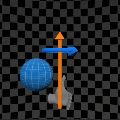
To determine the Positive Rotation, in three-Dimensional Euclidean Space we can use a hand rule similar to the one used for the cross-product.
The right-hand rule and left-hand rule in this context can be described as follows:
Bent fingers point in the direction of the Positive Direction, and your thumb indicates the axis of rotation
or
Point your thumb in the direction of the axis of rotation, and your bent fingers will indicate the Positive Direction.
Let us illustrate these rules using the following table:
| Left-Hand Axis of Rotation | Right-Hand Axis of Rotation |
|---|---|
 |  |
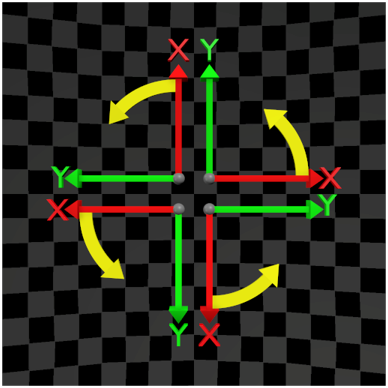
In three-dimensional Euclidean space, we encounter several possible permutations of basis vector orders. Fortunately, these permutations can be grouped into two groups of basis vector orders:
In the table below, I aim to demonstrate why the topic of the order of basis vectors—and, consequently, the Positive Direction of rotation—can appear complex and challenging to comprehend.
| Left-Hand Rule | Right-Hand Rule | |||
|---|---|---|---|---|
| -Up | 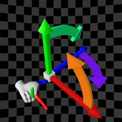 | 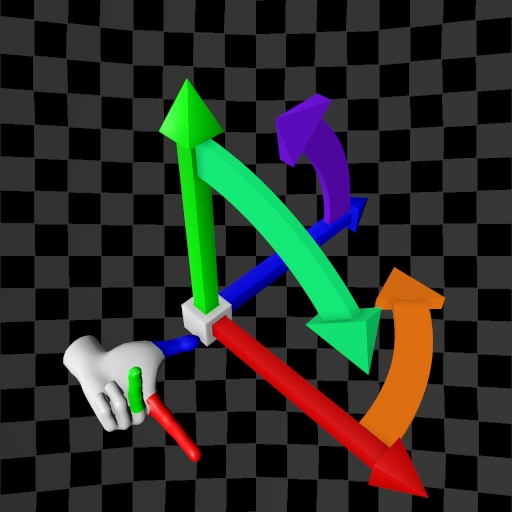 | 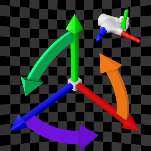 | 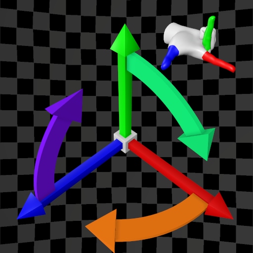 |
| -Up | 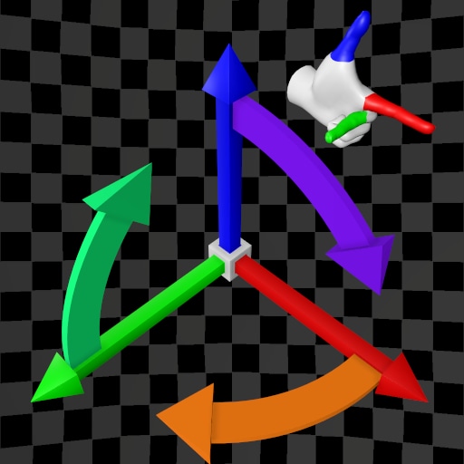 | 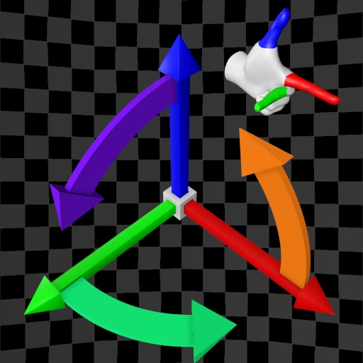 | 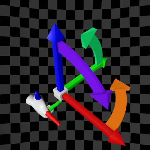 | 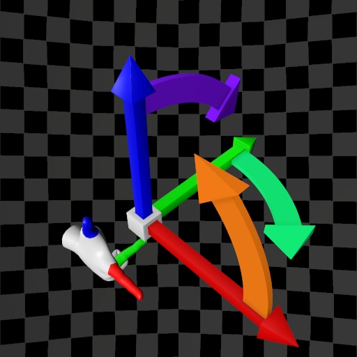 |
The variety of possible use cases increases the likelihood of making mistakes. How can we summarize the table above? After analyzing each case, the hand used to determine the order of the base vectors (and thus the Positive Direction of rotation), as well as the direction of the vector product, varies. In some cases, different hands are required, while in others, the same hand is used. The table below provides a summary of these cases:
| Basis Vector Order Group: | Basis Vector Order Group: | |
|---|---|---|
| Right-Hand Rule for Cross-Product | The SAME hand rule is used for both cross-product direction and Positive Direction | The OPPOSITE hand rule is used for cross-product direction and Positive Direction |
| Left-Hand Rule for Cross-Product | The SAME hand rule is used for both cross-product direction and Positive Direction | The OPPOSITE hand rule is used for cross-product direction and Positive Direction |
Maintaining coherence in basis vector order is essential for determining point positions in space and the Positive Direction of rotations. Only the basis vector order from the group satisfies these criteria.
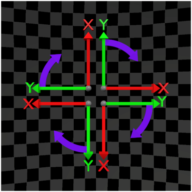
Finally, the Positive Direction in three-dimensional Euclidean space are illustrated in the table below:
| Left-Hand Rule | Right-Hand Rule | |
|---|---|---|
| -Up | 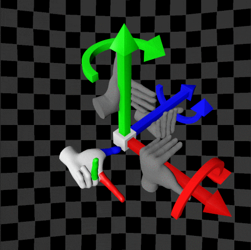 | 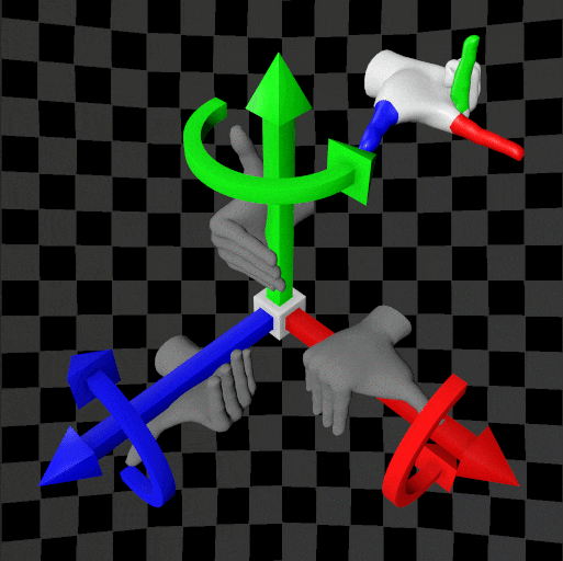 |
| -Up | 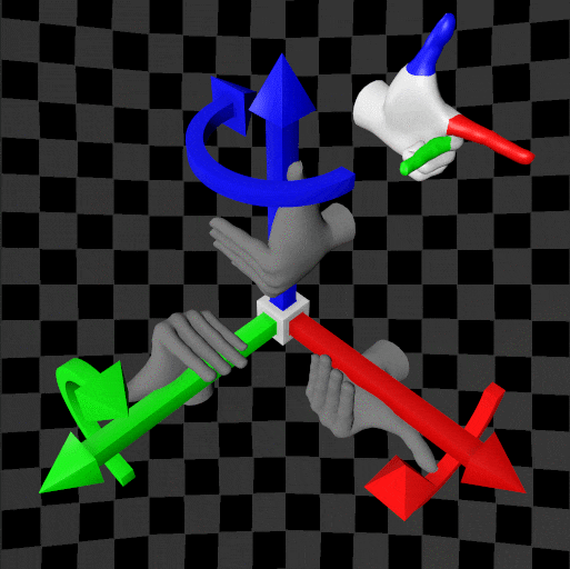 | 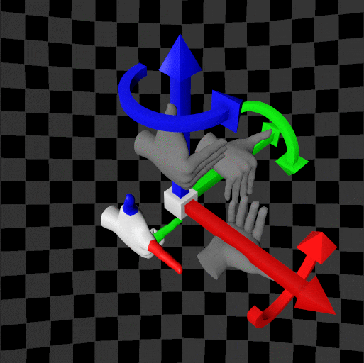 |
Consider this: If you create a model in a -Up left-handed coordinate system but render it in a -Up left-handed coordinate system, swapping the and coordinates may seem like a simple fix.
However, this adjustment implicitly alters elements like plane normal vectors, triangle mesh winding orders, and associated animation data due to changes in Positive Direction and basis vector order.
The order of basis vectors also affects quaternions. When W. R. Hamilton invented quaternions to describe rotations in three-dimensional Euclidean space, he defined them as and established dependencies between the imaginary components: , , , and . When quaternions are defined using these rules, the Positive Direction of rotation is determined by the right-hand rule. In computer graphics, however, there are applications that use the left-hand rule to determine the Positive Direction. This raises the question: how should quaternions defined in this manner be handled?
The convention proposed by M.D. Shuster does not change the fundamental definition of the quaternion itself but modifies its dependencies on the imaginary components. This approach differs slightly from the quaternion definitions typically found in mathematics textbooks. Notably, Shuster’s definition is employed by NASA’s Jet Propulsion Laboratory and, in computer graphics, within the Microsoft DirectX Math Library.
The differences between Hamilton’s and Shuster’s quaternion definitions are summarized in the following table:
| Hamilton’s Definition | Shuster’s Definition | |
|---|---|---|
| Imaginary Components Dependencies | ||
| Positive Direction | Determined by right-hand rule | Determined by left-hand rule |
| Matrix Multiplication Order | Post-multiplication | Pre-multiplication |
| “Sandwich” Product Order | ||
| Rotation Matrix |
To summarize Positive Direction concepts, here’s a table of applications (game engines or software tools for animations or models) that utilize different three-dimensional space orientations and specify the Up axis:
| Orientation | Left-Hand Rule | Right-Hand Rule |
|---|---|---|
| -Up | LightWave ZBrush Cinema 4D Unity | Autodesk Maya Modo Houdini 3D Animation Tool Substance Painter Marmoset Toolbag Godot OGRE |
| -Up | Unreal Engine* Open 3D Engine | Autodesk 3ds Max Blender SketchUp Autodesk AutoCAD CRYENGINE UNIGINE |
Unreal Engine uses both hand rules depending on the axis of rotation. For example:
and -Axis: Right-hand rule
-Axis: Left-hand rule
We now turn to a strictly implementation-related topic.
From the matrix definition, a matrix is a two-dimensional mathematical object (it has row and column dimensions), but computer memory operates linearly as a one-dimensional array.

How can we represent this matrix in computer memory?
A common solution is to use multidimensional arrays. These arrays can be mapped to computer memory in different ways, each offering distinct advantages and disadvantages.
The simplest and most widely used methods are the row-major and column-major conventions, where matrices are stored row by row or column by column, respectively.
| Row-Major | Column-Major | |
|---|---|---|
| Example Matrix |  | 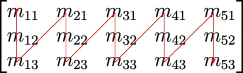 |
| Example Matrix |  | 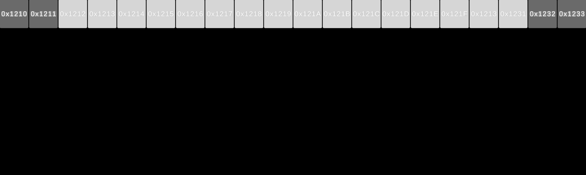 |
We have two conventions for storing matrices in memory, and each programming language must decide which one to adopt for its multidimensional array representation.
The following table summarizes how some popular programming languages implement these conventions:
| Storage Order | Programming Languages |
|---|---|
| Row Layout Order | C C++ Python (NumPy) Java Rust HLSL (by default or with GLSL (with |
| Column Layout Order | Fortran Matlab Julia HLSL (with GLSL (by default or with |
The majority of widely used languages favor row-major order, while those focused on numerical or scientific computations often prioritize column-major order.
Data storage conventions are inevitably linked to transformations.
For example, in a translation matrix, the translation vector is stored in either the third row or the third column, depending on the multiplication order.
| Pre-Multiplication | Post-Multiplication |
|---|---|
 |  |
Two multiplication orders and two storage conventions yield four ways to store a translation matrix:
| Pre-Multiplication | Pre-Multiplication | Post-Multiplication | Post-Multiplication |
| Row-Major | Column-Major | Row-Major | Column-Major |
|---|---|---|---|
 |  |  |  |
For performance reasons, it is better to read or write memory elements that are adjacent.
As a result, the translation vector should be stored using the convention that allows for this. This may explain why applications that store matrices in row-major order often prefer the pre-multiplication convention, while those storing matrices in column-major order tend to favor the post-multiplication convention.
But what can we do if, for some reason, we need to use the post-multiplication convention, and we don’t want to store matrices in column-major order?
There is a way—though somewhat hacky—but it is possible.
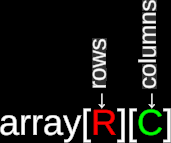
We can reinterpret the multidimensional array indices in a different order.
By doing this, in C/C++, we can pretend that the matrix is stored in column-major order rather than row-major order.
Both approaches to storing multidimensional arrays are summarized in the following table:
[Row][Column] Order | [Column][Row] Order |
|---|---|
foo[X][Y] is interpreted as matrix | foo[X][Y] is interpreted as matrix |
| To access matrix elements, specify the desired row using the first square bracket and the desired column using the second square bracket | To access matrix elements, specify the desired column using the first square bracket |
| The rows of a matrix correspond directly to the rows in a multidimensional array | The columns of a matrix correspond to the rows in a multidimensional array |
| More intuitive for mathematicians, as it aligns closely with the matrix definition | By doing this, we can pretend that matrices are being stored in column-major order |
 |  |
HLSL and GLSL shader languages are independent from the perspective of matrix multiplication and matrix storage. Similarly, hardware and Graphics APIs, such as DirectX® and Vulkan®, are also independent of these conventions and support various possibilities. However, their default behavior is defined by older API versions.
This independence is evident in how vectors and matrices interact. When a vector is multiplied by a matrix, , the vector is treated as a row vector. Conversely, when the matrix is multiplied by the vector, , the vector is treated as a column vector.
When 3D Graphics APIs were first introduced, they adhered to specific coordinate system conventions:
OpenGL®: Right-hand coordinate system, and a post matrix multiplication convention.
DirectX®: Left-hand coordinate system, and a pre matrix multiplication convention.
With the evolution of GPU hardware and graphics APIs, these conventions have become less rigid. Today, most APIs are agnostic to the coordinate system and multiplicative order, with two notable exceptions. The API must ultimately commit to (and cannot be overridden by the user) the handedness of the two and three-dimensional Euclidean space in the following contexts:
| API | Clipping Space |
|---|---|
| DirectX® | -Axis points to the right, -Axis points up, -Axis points into the screen, in the range |
| Vulkan® | -Axis points to the right, -Axis points down, -Axis points into the screen, in the range |
| OpenGL® | -Axis points to the right, -Axis points up, -Axis points into the screen, in the range |
| Metal | -Axis points to the right, -Axis points up, -Axis points into the screen, in the range |
| WebGPU | -Axis points to the right, -Axis points up, -Axis points into the screen, in the range |
| WebGL™ | -Axis points to the right, -Axis points up, -Axis points into the screen, in the range |
| API | Texture space |
|---|---|
| DirectX® | origin Top-Left corner, -Axis points to the right, -Axis points down |
| Vulkan® | origin Top-Left corner, -Axis points to the right, -Axis points down |
| OpenGL® | origin Bottom-Left corner, -Axis points to the right, -Axis points up (by default) |
| Metal | origin Top-Left corner, -Axis points to the right, -Axis points down |
| WebGPU | origin Top-Left corner, -Axis points to the right, -Axis points down |
| WebGL™ | origin Bottom-Left corner, -Axis points to the right, -Axis points up |
The above considerations—namely, the non-commutative nature of matrix multiplication and the anticommutativity of a vector’s cross product—have important consequences for the four alternative methods of constructing a 3D transformation as a 4×4 matrix. Each of these alternatives is described in detail in the sections below.
Pre-multiplication, left-handed coordinate system as in DirectX® 9
Post-multiplication, right-handed coordinate system as in OpenGL® 2
Transposing the entire 4×4 matrix will only change the pre- and post-multiplication order (without altering the coordinate system’s “handedness” or the order of the basis vectors).
Transposing just the upper-left 3×3 matrix will only change the order of the basis vectors (without affecting the pre- and post-multiplication order).
The specific convention used in an application may not be immediately apparent. Answering the following questions can help identify it:
Translation Matrix Construction: Examine how the components of the translation vector (, , ) are stored in memory. Are they stored adjacent to each other (1a) or separated (1b)?
Order of Transformations: Determine the sequence in which transformations (Scale, Rotation, and Translation) are applied. Is the composition executed as (2a) or (2b)? Similarly, is Matrix-Vector multiplication computed as (2a) or (2b)?
Rotation Storage: Check how rotation around the -Axis or -Axis is represented in memory. Does the first stored element correspond to (3a) or (3b)? For rotation around the -Axis, is the first stored element (3a) or (3b)?
Handedness of Coordinate System: Use the “hand rule” to determine the coordinate system. For the left hand, the straightened index finger points along the -Axis, the bent middle finger along the -Axis, and the extended thumb along the -Axis (4a). For the right hand, the corresponding directions are (4b).
With answers to these questions, the conventions in use can be identified using the table below.
| Question 1 | Question 2 | Question 3 | Question 4 | Convention | |
|---|---|---|---|---|---|
| 1a | 2a | 3a | 4a | Post-multiplication, Column-Major, , Left-handed | |
| 1b | 2a | 3a | 4a | Post-multiplication, Row-Major, , Left-handed | |
| 1a | 2b | 3a | 4a | Pre-multiplication, Row-Major, , Left-handed | |
| 1b | 2b | 3a | 4a | Pre-multiplication, Column-Major, , Left-handed | |
| 1a | 2a | 3b | 4a | Post-multiplication, Column-Major, , Left-handed | |
| 1b | 2a | 3b | 4a | Post-multiplication, Row-Major, , Left-handed | |
| 1a | 2b | 3b | 4a | Pre-multiplication, Row-Major, , Left-handed | |
| 1b | 2b | 3b | 4a | Pre-multiplication, Column-Major, , Left-handed | |
| 1a | 2a | 3a | 4b | Post-multiplication, Column-Major, , Right-handed | |
| 1b | 2a | 3a | 4b | Post-multiplication, Row-Major, , Right-handed | |
| 1a | 2b | 3a | 4b | Pre-multiplication, Row-Major, , Right-handed | |
| 1b | 2b | 3a | 4b | Pre-multiplication, Column-Major, , Right-handed | |
| 1a | 2a | 3b | 4b | Post-multiplication, Column-Major, , Right-handed | |
| 1b | 2a | 3b | 4b | Post-multiplication, Row-Major, , Right-handed | |
| 1a | 2b | 3b | 4b | Pre-multiplication, Row-Major, , Right-handed | |
| 1b | 2b | 3b | 4b | Pre-multiplication, Column-Major, , Right-handed |