RPS Tutorial Part 2 – Exploring Render Graphs and RPSL
Introduction
In the previous tutorial, we learned how to make a simple application where a single triangle was rendered to the screen. In this tutorial part, we will answer key questions regarding RPSL, and we’ll develop a deeper understanding of the RPS render graph.
Overview
Resources in render graphs
In the tutorial introduction, it was briefly mentioned that the RPS SDK provides an elegant and efficient solution to managing transient memory. This takes the form of transient resources that we may easily create within our render graphs.
An example of transient resources would be something like the following,
compute  node tone_mapping([readwrite(cs)] texture src);graphics node blt_swapchain_color_conversion(rtv rt : SV_Target0, srv src);
export void rps_main([readonly(present)] texture backbuffer){    ResourceDesc backbufferDesc = backbuffer.desc();    uint32_t width = (uint32_t)backbufferDesc.Width;    uint32_t height = backbufferDesc.Height;
    texture colorBuffer = create_tex2d(RPS_FORMAT_R16G16B16A16_FLOAT, width, height);    clear( colorBuffer, float4(0, 0, 0, 0) );
    // do work ...
    tone_mapping(colorBuffer);    blt_swapchain_color_conversion(backbuffer, colorBuffer);}
The create_tex2d built-in node declares a resource as part of the render graph description that the RPSL program specifies. The return value of create_tex2d is a default resource view on the declared resource.
We’ll drill down this point again, resource views are the working flux of RPS. To further specify a view from the default one, we can create derived resource views. This is done via member functions on either the texture or buffer view types. For example, .mips can be used to create a view with a subresource range over a range of texture mips. For the full listing of such member functions, please see rpsl.h.
The RPS SDK automatically creates and destroys these transient resources within graphics API heaps; it can also efficiently alias such resources, reducing total memory usage. Again, the creation of these transient resources, like the invocation of nodes, is virtual. They get created after the execution of the RPSL program and during the render graph update.
As for the C API side, rpsRenderGraphDeclareResource can be called from within the build callback to declare a transient resource.
RpsResourceId rpsRenderGraphDeclareResource(RpsRenderGraphBuilder hRenderGraphBuilder, const char* name, RpsResourceId localId, RpsVariable hDesc);The fourth parameter of this call is meant to be a pointer to the resource description, which should be of type RpsResourceDesc. The localId must be unique per render graph for every declared resource. Undefined behavior occurs if two calls have the same localId and are made within the same build callback. When making subsequent render graph build calls that refer to this resource, the RpsResourceId returned from the original call must be used.
In general, for reference on building a render graph via the C API, a concrete example can be found in test_builder_c.c.
Resource classes
In the previous section, it was mentioned that only transient resources are managed by the RPS runtime. However, this holds true for any resource declared from within the render graph. Indeed, transient resources are not the only class of resource.
There are other types of resources that render graphs can work with. The total list of resource types are: external resources; persistent resources; transient resources; and of course, as mentioned in the first tutorial part, temporal resources.
An external resource is any resource that is passed into the render graph via the entry node. This includes output resources, which are discussed in detail within the faq.md.
Persistent resources are those whose data persists (unless explicitly cleared) across render graph updates. A transient resource is any resource that is not persistent.
We can create a persistent resource via the RPS_RESOURCE_FLAG_PERSISTENT resource flag,
export void rps_main([readonly(present)] texture backbuffer){    ResourceDesc backbufferDesc = backbuffer.desc();
    texture lastFrame = create_tex2d(        backbufferDesc.Format, backbufferDesc.Width, backbufferDesc.Height, 1, 1, 1, 1, 0, RPS_RESOURCE_FLAG_PERSISTENT);
    // do work ...
    copy_texture(lastFrame, backbuffer);}
A helpful way to think about persistent resources is as similar to static variables on the CPU side. Such variables are initialized only once, but then at a later time may be set to another value. Persistent resources go along the same lines – the creation occurs only once, and until the resource description changes through the call to create_tex2d, the resource data persists.
Both external resources and temporal slices are implicitly persistent resources. External resources are obviously so, and if temporal resources weren’t, it would be impossible to access historical slices.
RPS render graph structure
As mentioned in the first part, a render graph takes the form of a linear sequence of nodes to call. We also know that this sequence is reordered by a scheduler phase. Further, we know that there are these things called graph commands that we iterate over when recording.
This prior discussion was leaving out some important details and doesn’t quite paint the full picture. The scheduler phase is just one phase of an entire set of render graph phases. And therefore, a render graph takes on many different forms as the phases run – particularly, and as we would expect, it takes on a much more complicated graph structure than a mere linear sequence.
Render graph build phases
Here’s how the render graph gets transformed by the phases:
It begins as a linear, ordered sequence of command nodes, with the same order as specified in the shader. Command nodes are cached calls to declared or built-in nodes, where the parameter values are saved. The first phases take in this sequence and transform it into a directed acyclic graph, making connections and inserting new nodes where needed. From there, the work of the scheduler phase slots all the DAG nodes into a linear sequence of what are called runtime commands (these are the previously denoted graph commands). Runtime commands are simply command nodes (or any of the nodes that were newly inserted) that have been decidedly scheduled to be recorded by the runtime backend; some runtime commands may be eliminated during the scheduler phase if deemed to have no side effect.
Not all of the phases manipulate the render graph. Some of them are there for debugging purposes, of which there are three: CmdDebugPrintPhase, DAGPrintPhase, and ScheduleDebugPrintPhase. The first phase prints out the priorly mentioned program-order sequence of command nodes. This is the form before any of the render graph phases manipulate the structure of the render graph. The second phase prints out the DAG in the DOT language such that it could be rendered with e.g. Graphviz or some other graph visualization software. The final print phase prints the result of the scheduler phase; i.e., it prints the linear stream of runtime commands that is ultimately iterated over by the host app to record API commands to some command buffer.
What the render graph means and how it works
Now that we know about how the thing is built, we can begin to discuss the structure and meaning of it.
Consider the picture below of an RPS DAG from our MRT test (found at test_mrt_viewport_clear.rpsl):
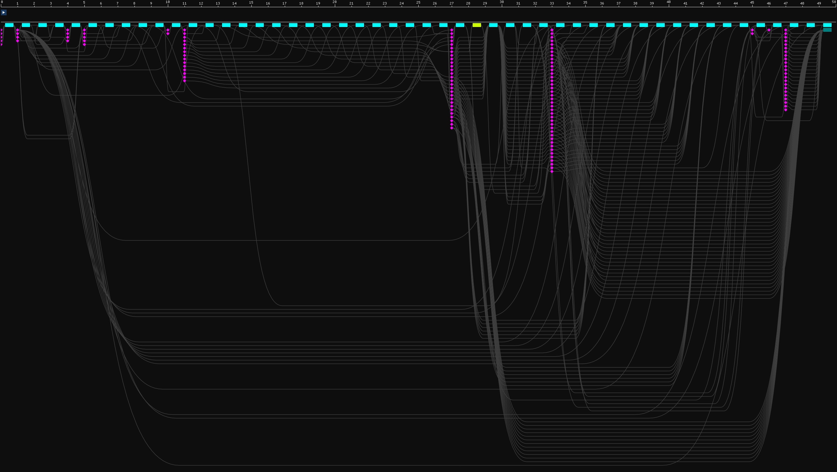
The ruler at the top is the timeline, denoting the indexes of commands to record. The commands to record are visualized as the rectangles below the ruler. These commands are nodes from the graph that have been slotted, with the DAG edges retained for visualization purposes. The colors of the commands signify minimum queue families such as graphics (cyan), compute (orange), and copy (lime). These colors are used RPS-SDK wide.
If you weren’t already aware, this SDK ships with a useful tool for navigating RPS render graphs – the RPSL Explorer. It was used to generate the image above and can be found at /tools/rpsl_explorer. The explorer works by integrating a separated visualizer library, which can visualize resource lifetimes, heap allocations, and the render graph itself. It is a good idea to hook this into your engine to access the same visualization capabilities. The lib can be found here: /tools/rps_visualizer/.
Okay, we know what we are looking at. But, what does it mean?
The edges indicate an ordering dependency between nodes, i.e., when the scheduler pass slots nodes into the linear command stream, it must obey that the work in some node A is to be submitted to the GPU before the work in some node B.
As for the meaning of the nodes themselves, it goes like so:
Unless otherwise specified, any writes by a node in the graph are guaranteed to appear as if they executed on the GPU atomically. The scope in which to consider the operation atomic is within the set of nodes in the graph that access the same subresource. This guarantee is due to two implicit and conceptual memory dependencies: one before the node access and one after it.
Here, the definition of memory dependency is similar to that in the Vulkan specification. When both the begin/end dependencies are considered, it can be said that writes by a node happen before and are made both available and visible to subsequent node accesses, and that they happen after previous readonly node accesses.
Another element of synchronization is between render graph executions, i.e., the scope of synchronization for any write to a persistent resource by a node is not just within a single render graph execution but within the entire sequence of render graph executions across time.
In the case where the host app records work to be done on external resources from outside of a node callback, synchronization may also be required. Recall that the access attributes for entry node parameters (external resources) establish how the resource is accessed outside the scope of the graph. Thus, if either the outside scope or accesses within the graph write to an external resource, synchronization is required.
We’ll close with what all this means pragmatically:
A render graph enables its conceptual model and that of a node via the insertion of transition nodes. These are the purple diamonds in the image above, and they are scheduled as batches between the runtime command rectangles. When recording the render graph and iterating over a batch of transitions, those transitions are recorded to the command buffer as explicit API barriers (unless the runtime backend in use does not support them).
Render graph node dependencies
Thus far, we understand that every write access by a node to a resource is synchronized with every other access to that resource. We’ve also mentioned that every edge in the graph indicates a submission order dependency between two nodes.
But, in what cases are graph edges inserted?
This occurs if for two subsequent command nodes, at least one of them contains a write access to the same subresource. Edge insertion also occurs when the runtime backend considers subsequent accesses to require a transition between them. As an example, the Vulkan runtime backend requires that subsequent accesses to the same subresource of [readwrite(copy)] require a transition. Finally, there is a set of general cases for which edge insertion can occur, such as back-to-back UAV accesses.
The render graph data flow model
To complete this section, we’ll provide an elegant conceptualization of all the aforementioned rules.
As a consequence of the synchronization of write nodes and the condition for when graph edges are inserted, we can logically deduce that the edges of a render graph denote data flow between graph nodes. Here, “data flow” is how data is considered to be temporally accessed by nodes across a frame during execution on the GPU. For any incoming edge into a node, the associated work within the node callback for that edge cannot appear to have begun until the incoming data has “arrived” at the node.
Exploring RPSL
Access attributes
As mentioned in the first tutorial part, every parameter of every node may be decorated with something called access attributes. Access attributes describe a particular type of access that a node views some resource with. The general form includes any of readonly, writeonly, and readwrite, followed by attribute arguments contained within ().
technically, none of readonly (RO) / writeonly (WO) / readwrite (RW) need be present and an attribute such as [relaxed] is entirely permissible. See faq.md for more details on the [relaxed] attribute. It is also possible to specify access attributes in an unordered list, for example, [relaxed] [readwrite(ps, cs)].
readonly, writeonly, and readwrite are exactly as they sound, i.e., they control whether the node is permitted to read, write, or both read and write to a resource. The writeonly access attribute has an additional clause which is that it indicates that the previous data of the viewed subresource range can be discarded. Such a clause implies the following equality relation, writeonly = readwrite(discard_before).
Access attribute arguments
discard_before is an attribute argument indicating that this view access by the node doesn’t care about the data before and therefore the data may be discarded. discard_after is a symmetric argument and works in the opposite way. Formally, these are data dependency indicators. RPS is free to ignore them or otherwise use them for optimization purposes.
Since these are data dependency indicators and not strong directives, it’s easy to see that something like readonly(discard_before) on some node parameter could never map to a discard recorded by that node. Such a discard constitutes a write, and of course, a readonly access on a view may not write to the viewed resource. For discard arguments to readonly attributes, a discard operation would only be recorded if any surrounding runtime command nodes have write access to the same subresource range. This is because if some runtime command has an attribute with discard_before, RPS may patch a previous command if appropriate with discard_after.
The other sort of attribute arguments describe a particular access type. The example discussed in the first tutorial part was rendertarget. It was explained that nodes accessing the resource with this access would ensure the resource is able to be accessed as a render target view by the node, and that this results in potential state/layout transitions by the runtime backend. In general, all of what would be required as per the graphics API to access this resource as a render target view is handled by the RPS runtime. This means that for example on the DX12 side, the resource must be created with D3D12_RESOURCE_FLAG_ALLOW_RENDER_TARGET.
So in fact, there is an additional contract between the user and RPS. When providing external resources, you need to ensure that the resource can be accessed as per how it is used in the render graph.
Aside from a particular access type, attribute arguments are also used to specify pipeline stages the resource is to be accessible by. For example, one of the snippets used above was [readwrite(ps, cs)], which indicates that the viewed subresource range is accessible by the pixel and compute shader pipeline stages. These access attribute types are used e.g. by some runtime backends to establish the appropriate synchronization scopes to use within explicit API barriers.
To see the documentation for all attribute arguments, please see rpsl.h.
Modular RPSL
There are two primary methods to achieve modularization within RPSL:
-
HLSL functions.
-
Composing render graphs.
Again, the render graph command nodes are the set of nodes that during the execution of the RPSL program were noted to be called. There is no requirement that nodes must be called within the entry function for the program – things work just fine if they were from within some HLSL function that is not the entry.
Consider for example,
void foo(){    nodeA();    nodeB();    nodeC();}
entry void main([readwrite(present)] texture backbuffer){    foo();}
The example above produces a graph with with command nodes of A, B, and C.
As for composing render graphs, this means to bind entire graphs to node callbacks. This can be done by making a call to rpsProgramCreate to create an RpsSubprogram from an arbitrary RPSL entry point, then binding that subprogram as a node callback via rpsProgramBindNodeSubprogram. Composing render graphs has the effect of “inlining” the subordinate program; “inlining” means that during the execution of the primary RPSL program, instead of noting the node to be called, the subprogram RPSL entry is invoked, thereby contributing to the total set of command nodes that constitute the render graph. A detail to keep in mind is that the info for what callback to invoke for a node when recording the graph is stored within an RpsSubprogram, which means that binding callbacks to node declarations is to be done on a per program basis. This means that two programs can share a single node declaration yet runtime commands of that node decl can invoke different callbacks based on the program that the node was part of.
For an example, please see test_subprogram_d3d12.cpp.
Tools for scheduling
For fine granularity control of the ultimately scheduled command stream, RPSL offers various tools for scheduling.
sch_barrier():
This is a scheduling intrinsic that can be used to create a barrier that no nodes can be scheduled over. It forms a set of nodes A before the barrier and a set of nodes B after the barrier such that no nodes from set A may be scheduled after the barrier, and no nodes from set B may be scheduled before the barrier.
Here’s an example,
{ // this will never be scheduled as nodeB -> nodeA. nodeA(); sch_barrier(); nodeB();}sch_barrier() is useful if e.g. some “setup” node must be recorded first. Maybe the node has side effects on the host app side that affects the behavior of any subsequent node callbacks, but otherwise does not access any resources. Such a node would be free from the perspective of the scheduler to exist anywhere in the command stream, but as developers this is understood to be required to occur before all other nodes.
[subgraph(atomic, sequential)]:
This is an attribute that can be applied to an HLSL function or a scope. The heading above notes the attribute arguments of atomic and sequential. When the subgraph attribute is applied to a scope, all nodes within the scope are within the subgraph, whereas when it is applied to an HLSL function, this results in all nodes that get called as a result of calling that function as being within the subgraph.
The sequential argument indicates that the relative order of the nodes within the subgraph are retained. Consider for example,
{ [subgraph(sequential)] { nodeC(); nodeB(); nodeA(); } nodeD();}In the example above, the scheduler will never reorder the relative sequence of nodeC -> nodeB -> nodeA. However, nodeD may still be inserted into the scope of the subgraph (e.g. forming a runtime command stream such as nodeC -> nodeD -> nodeB -> nodeA).
The atomic argument means that nodes outside the subgraph cannot be rescheduled into the scope of the subgraph, and vice versa. A potentially useful mental model for atomic subgraphs is to consider them as being functionally replaceable with a single node. This node would have a parameter for each element in the set of resources that get accessed by the nodes of the subgraph, and its callback would include and string together all the subgraph work via internal transitions.
Subgraphs can also be specified recursively,
{ [subgraph(sequential)] { [subgraph(atomic, sequential)] { nodeB(); nodeC(); } [subgraph(sequential)] { nodeD(); nodeE(); } nodeA(); }}When subgraphs are nested, this forms a tree structure where the leaf nodes are the node calls, such as in the example above with nodeB(), nodeC(), etc. When the root node is a sequential subgraph, the sequential attribute argument doesn’t apply to the immediate children but rather applies to the relative ordering of the leaf nodes. Therefore, the example above would schedule to a fixed relative ordering of B -> C -> D -> E -> A.
async:
To allow for asynchronous compute scenarios, the async keyword can be used to hint that work should be scheduled on a queue that is not the main graphics one. This keyword is used as part of the expression when calling a node.
Consider e.g. the following line of RPSL,
async Procedural(proceduralTex, cbView, uint2(proceduralTexWidth, proceduralTexHeight));This keyword is ignored when used with a call to a graphics node.
HLSL semantics
Thus far, HLSL semantics such as SV_Viewport[n], SV_ScissorRect[n], and SV_Target[n] have already been mentioned as RPSL keywords that can be used to decorate node parameters for the purpose of automatically setting up viewport rects, scissor rects, and render targets, respectively, in the command callback.
Other semantics for binding targets exist and these are SV_DepthStencil and SV_ResolveTarget[n]. These may be used to bind a depth/stencil buffer and resolve targets, respectively. For example,
node draw(rtv rt : SV_Target0, [readwrite(depth, stencil)] texture ds : SV_DepthStencil);node draw_msaa(rtv rtMSAA : SV_Target0, [writeonly(resolve)] texture rt : SV_ResolveTarget0);Access attributes such as depth, stencil, and resolve do nothing in terms of automatic setup in the callback. These are merely to establish the access type that this node may access the resource view by. The SV_DepthStencil semantic, in a separate manner, controls the binding of the depth/stencil buffer, such that there is no need to do so in the callback for draw. In the DX12 backend, this is done via OMSetRenderTargets, whereas in the Vulkan backend a render pass with the appropriate attachment is created and begun.
As for the behavior of SV_ResolveTarget[n], this must be used when the node already has some SV_Targets too, i.e., SV_ResolveTarget[n] converts what would otherwise have been a regular render pass to a render pass that culminates in the resolve of the render targets to the resolve targets. The resolves are automatically recorded after the host application node callback returns. To simply perform a resolve without attaching it to an existing node, there exists a built-in resolve node. Of course, nothing is stopping a developer from implementing a custom resolve node should they chose to do so.
Additional semantics such as SV_ClearColor[n], SV_ClearDepth, and SV_ClearStencil can be used to instruct RPS to clear the associated convenience bound targets.
We’ll demonstrate this with some snippets below,
node clear_targets(rtv rt0 : SV_Target0, rtv rt1 : SV_Target1, rtv rt2 : SV_Target2, dsv ds : SV_DepthStencil, // dsv = [readwrite(depth, stencil)] texture float4 clearColor0 : SV_ClearColor0, float clearDepth : SV_ClearDepth, uint clearStencil : SV_ClearStencil);When invoking the clear_targets node above, we may provide the values to clear to,
const uint w = 1280;const uint h = 720;
texture rt0  = create_tex2d(RPS_FORMAT_R8G8B8A8_UNORM, w, h);texture rt1  = create_tex2d(RPS_FORMAT_R16G16B16A16_FLOAT, w, h);texture rt23 = create_tex2d(RPS_FORMAT_B8G8R8A8_UNORM, w, h, 1, 2);texture ds   = create_tex2d(RPS_FORMAT_R32G8X24_TYPELESS, w, h);
clear_targets(rt0, rt1, rt23.array(0), ds.format(RPS_FORMAT_D32_FLOAT_S8X24_UINT), float4(0, 1, 0, 1), 0.5f, 0x7F);
Similar to the setup of viewport and scissor rects, these clears occur before the host callback is invoked.