Occupancy explained

If you’re working with GPUs, chances are you’ve heard the term occupancy thrown around in the context of shader performance. You might have heard it helps hiding memory latency but are not sure exactly what that means. If that’s the case, then you are exactly where you should be! In this blog post we will try to demystify what exactly this metric is. We will first talk a bit about the hardware architecture to understand where this metric is coming from. We will then explain the factors that can limit occupancy both statically at compile time and dynamically at run time. We will also help you identify occupancy-limited workloads using tools like the Radeon™ GPU Profiler and offer potential leads to alleviate the issues. Finally, the last section will try to summarize all the concepts touched upon in this post and offer practical solutions to practical problems.

This article however assumes you have a basic understanding of how to work with a GPU. Mainly, we expect you to know how to use the GPU from a graphics API perspective (draws, dispatches, barriers etc.) and that the workloads are executed in groups of threads on the GPU. We also expect you to know about the basic resources a shader uses like the scalar registers, vector registers, and shared memory.

GPU workload distribution

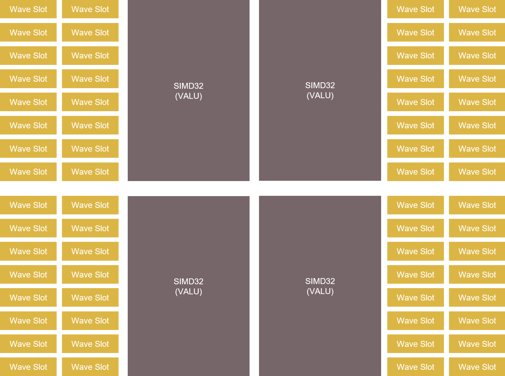
To understand the concept of occupancy we need to remember how the GPU distributes work. From the architecture of the hardware, we know that the computing power of the GPU lies in the Single Instruction Multiple Data (SIMD) units. The SIMDs are where all the computation and memory accesses in your shader are processed. Because the SIMD datapaths in AMD RDNA™-based GPUs are 32-wide, the GPU executes workloads in groups of at least 32 threads, which we call a wavefront, or wave for short. For any given overall workload size, the GPU will break it into wavefronts and dispatch them to the available SIMDs. There will often be more wavefronts to run than available SIMDs, which is fine because each SIMD can have multiple wavefronts assigned to it. From now on, we will refer to the action of assigning a wave to a SIMD as launching a wave. In RDNA1, each SIMD has 20 slots available for assigned wavefronts, and RDNA 2 and RDNA 3 have 16 slots per SIMD.

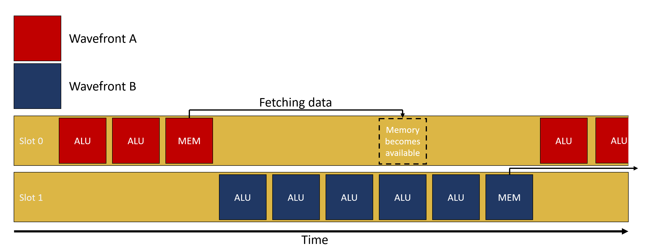
While multiple wavefronts can be assigned to a single SIMD, only one wavefront can be executed at a time on this SIMD. However, the assigned wavefronts don’t have to be executed in order and they don’t have to be fully executed in one go either. This means that the GPU is free to execute any assigned wavefront on a given SIMD and can do so cycle-by-cycle, switching between them as needed, as they execute.

It makes that possible by knowing what each shader is doing by tracking wavefront execution, giving it a view of what’s currently running, what resources are being used and are available, and knowing what could run next. Its main job by doing that is to hide memory latency, because accessing external memory in a shader is costly and can take hundreds of clock cycles if the access is not cached. Rather than pause the running wavefront and wait for any memory access, cached or not, because it’s managing multiple assigned wavefronts it can pick and start another one in the meantime.

Let’s take an example, wavefront A is picked up by the SIMD, starts running some ALU computations and at some point, needs to fetch data from memory (e.g. sample a texture). Depending on how recently this data was accessed, the request might go through the entire cache hierarchy, go into memory, and finally come back. This might take up to a few 100s of cycles and without multiple wavefronts in flight, the SIMD would just wait for the data to come back. With multiple wavefronts in flight, instead of waiting for the results to come back, the GPU can simply switch to a different wavefront, let’s say wavefront B, and execute it. Hopefully, wavefront B starts by doing some ALU computations before requiring itself data from memory. All those cycles spent on running ALU computations from wavefront B are hiding the latency of fetching data for wavefront A. If there are enough wavefronts in flight which have ALU operations to execute, it is possible for the SIMD to never be idle.

One way to visualize the impact of latency hiding is to use the Radeon GPU Profiler (RGP) and inspect the instruction timings of a single draw or dispatch. In the following image, we’re looking at the instructions executed by the GPU. In the latency column we can see for each instruction how many clocks it took to execute. If we look at instruction 435, we can see that it took about 8.5 million clocks in total. Because it’s a memory wait instruction, we want to spend as little time as possible actually stalled waiting and instead hide that latency by switching to a different wavefront. This is exactly what the color coding is showing us. The first part of the bar, of which about 80% is colored green, means that about 80% of the overall time spent waiting was actually hidden by executing vector ALU operations from different wavefronts instead. We can also see that at the beginning of the green bar there are some yellow hatching lines, meaning scalar ALU operations were also executed in parallel to those vector ALU operations.

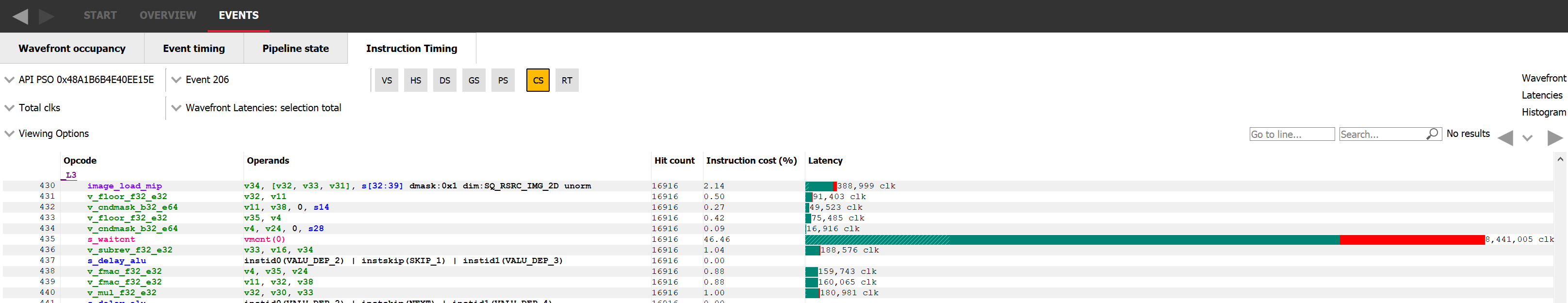
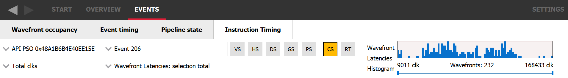
On a side note, this tab also shows the repartition of the length of the analyzed wavefronts as a histogram. This visualization helps you realize that the execution length of different wavefronts can and does vary greatly within a single workload. It is also possible to isolate some wavefronts for instruction timing analysis by selecting a region of the histogram using the widget directly underneath it.

This wavefront switching mechanism only works if the GPU is able to switch the running wavefront quickly; the overhead of switching must be lower than the potential time the SIMD would spend idle. To switch swiftly, all of the resources that the wavefronts need are made available at all times. That way, when switching to a different wavefront, the GPU can immediately access the required resources for it to run.

Occupancy definition

Occupancy is the ratio of assigned wavefronts to the maximum available slots. In RDNA2 onwards, for a single SIMD, this means the number of assigned wavefronts divided by 16. Let’s take an example, if a SIMD has 4 wavefronts in flight, the occupancy is 4 / 16 = 25%. A different interpretation of occupancy is the capacity of the SIMD to hide latency. If the occupancy is 1 / 16, it means that if the wavefront has to wait for something, the latency cannot be hidden at all since no other wavefront is assigned to this SIMD. On the other end of the spectrum, if a SIMD has an occupancy of 16 / 16, it is in good position to hide latency.

Before diving deeper into occupancy, now might be a good time to get some intuition on when latency hiding, and thus occupancy, correlates with performance. Since increasing occupancy means increasing the latency hiding capacity of the GPU, a workload that is not latency bound will not benefit from increased occupancy. An example of this would be an ALU bound workload. We don’t need to increase the number of available waves per SIMD if it is already running at 100% utilization and not spending any time waiting for something.

If we put it the other way around, the only workloads that might benefit from increased occupancy are the ones latency bound. Most workloads will follow the following pattern: load data, do some ALU work on it, store data. So a workload that could benefit from adding some more waves would be one where the number of waves multiplied by the time it takes to run the ALU work is lower than the time it takes to load the data. With more waves in flight, we increase the amount of overall ALU work available to hide the latency from loading the data.

That being said, occupancy is not a silver bullet and can also decrease performance. In heavily memory bound scenarios, increasing the occupancy might not help, especially if very little work is being done between the load and store operations. If the shader is already memory bound, increasing the occupancy will result in more cache trashing and will not help hide the latency. As always, this is a balancing act.

Theoretical occupancy

So far we have described occupancy as a consequence of an internal scheduling mechanism, so let’s talk about the specific components that can affect that. As mentioned earlier, to be able to quickly switch between wavefronts the SIMD reserves in advance all the required resources to run all the assigned wavefronts. In other words, the GPU can only assign wavefronts to a SIMD if enough resources are available for them to run. In general, those resources are the Vector General Purpose Registers (VGPRs), the Scalar General Purpose Registers (SGPRs) and the “groupshared” memory, which we call the Local Data Share (LDS). On RDNA GPUs however, each wavefront is assigned a fixed number of SGPRs and there are always enough of those to fill the 16 slots.

The amount of resources required by a shader to run on a SIMD is evaluated at compile time. The shader compiler stack will compile the high-level code (HLSL, GLSL etc.) to GPU instructions and assess how many GPRs and how much LDS is required for the shader to run on a SIMD. On RDNA GPUs it will also make a decision about whether the shader should run in the native wave32 mode, or in wave64 mode where the wavefront contains 64 threads. Wave64 shaders run each wavefront over 2 cycles, and have higher resource requirements, as you might guess.

For compute shaders, the threadgroup size is another factor in the theoretical occupancy. When writing a compute shader, the user must define the number of threads that will execute as a group. This is important because all the threads of a single threadgroup can share data through some shared memory called Local Data Share (LDS). In RDNA-based GPUs, the LDS is part of the Work Group Processor (WGP). This means that all the threads from a single threadgroup have to execute on the same WGP, otherwise they wouldn’t be able to access the same groupshared memory. Note: this restriction only applies to compute shaders. In general, not all wavefronts that are assigned to a single SIMD need to be part of the same draw or dispatch.

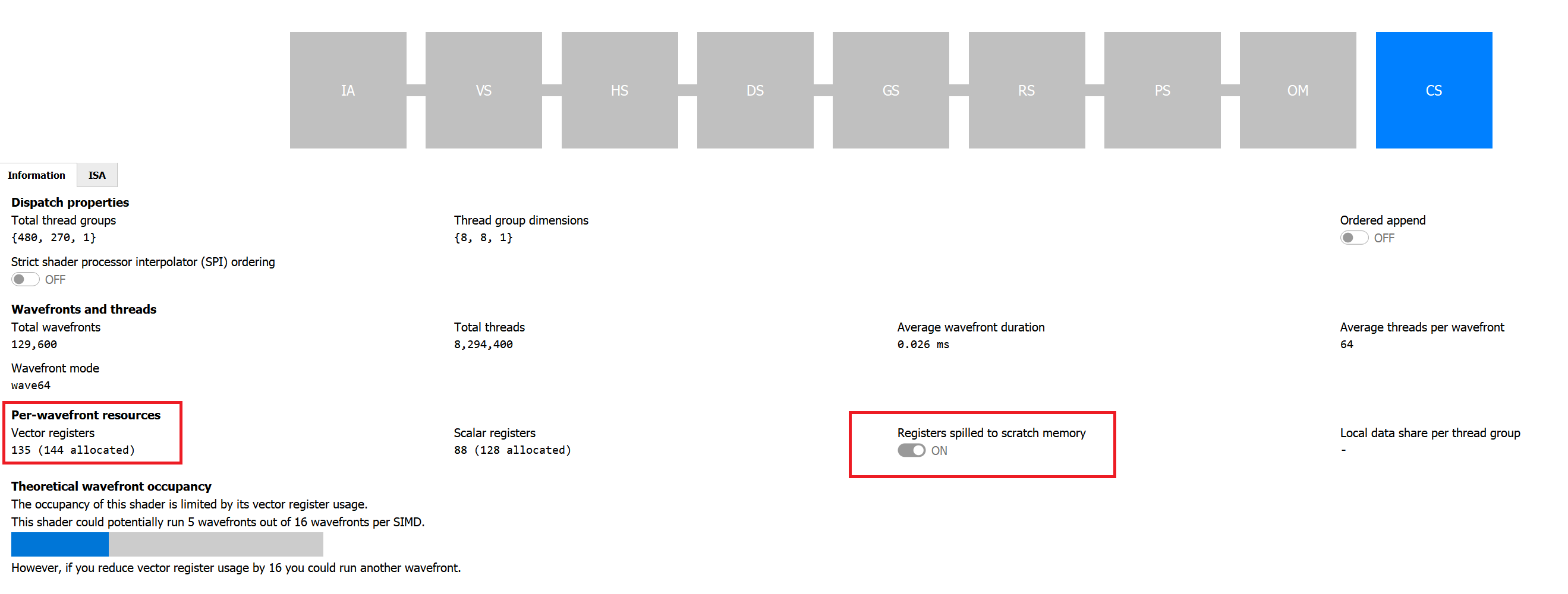
Using all those constraints, it is possible for you to calculate the theoretical occupancy of a shader on a given GPU and know which resource might be limiting it, but we make that easy in Radeon GPU Profiler (RGP) on the pipeline tab, as shown in the following image. It indicates the current theoretical occupancy, which resource is the limiting factor, and by how much it needs to be reduced to increase the occupancy by 1. If you’re willing to do the computation by hand, the pipeline tab still shows how many resources are required by the shader, which wave mode it is running in, and the threadgroup size if it is a compute shader.

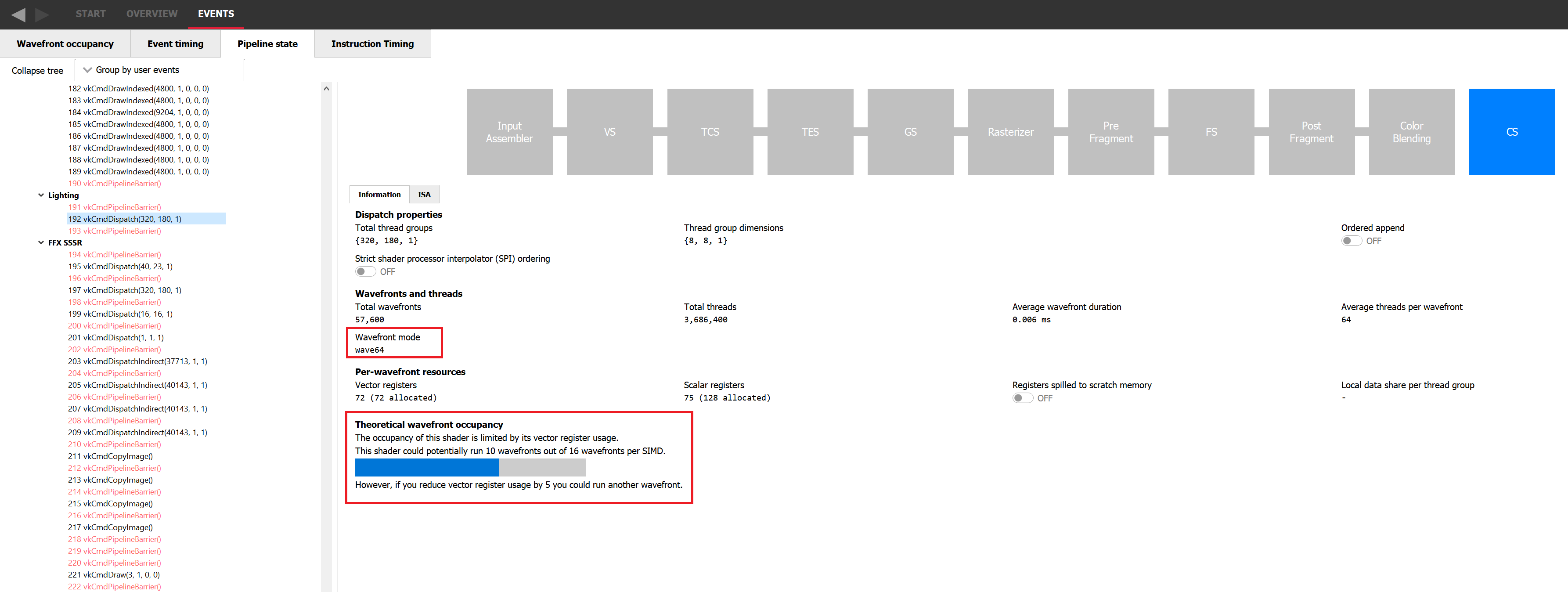
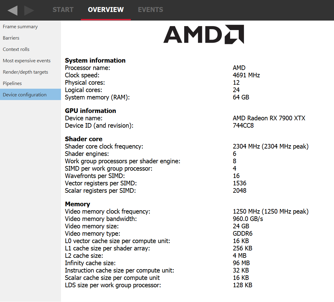
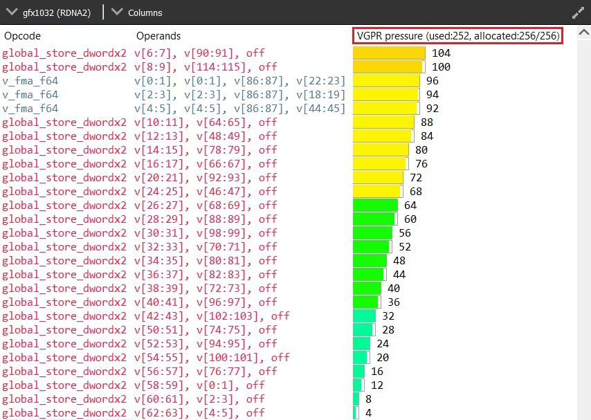
Let’s take an example where the theoretical occupancy is limited by VGPR pressure. For instance, let’s consider a shader that requires 120 VGPRs and is not limited by LDS otherwise. If we go to the device configuration tab of RGP we can see that for the AMD Radeon RX 7900 XTX GPU, there are 1536 VGPRs available per SIMD. This means that in wave32 mode, since 1536 / 120 = 12.8, we can assign 12 wavefronts to a SIMD. This also means that in theory, for a shader that requires only 118 VGPRs, 13 wavefronts can be assigned. In practice, VGPRs have allocation granularity greater than 1, and so that shader would need to request less than 118 VGPRs to be assigned 13 times. The size of a block depends on the architecture and wave mode but RGP will tell you exactly how many VGPRs you need to save to be able to assign a new wave. In wave64 mode, we would need to save even more VGPRs to be able to assign one more wavefront.

Understanding where the register pressure is coming from is not an easy task without the proper tools. Fortunately, Radeon GPU Analyser (RGA) is here to help. RGA lets you compile shaders from high-level source code into AMD ISA and provides insight into the resulting resource requirements. For instance, it can display how many VGPRs are alive for each instruction of the program at the ISA level.

This kind of visualization is very helpful to identify potential VGPR usage spikes in a particular shader. Because the GPU allocates for the worst case requirements in the shader, a single spike in one branch of the shader can cause the entire shader to require a lot of VGPRs, even if that branch is never taken in practice. For more information on how to use RGA, please check the dedicated GPUOpen RGA page and our guides on Live VGPR Analysis: Live VGPR analysis with RGA and Visualizing VGPR pressure with RGA.

Measured occupancy

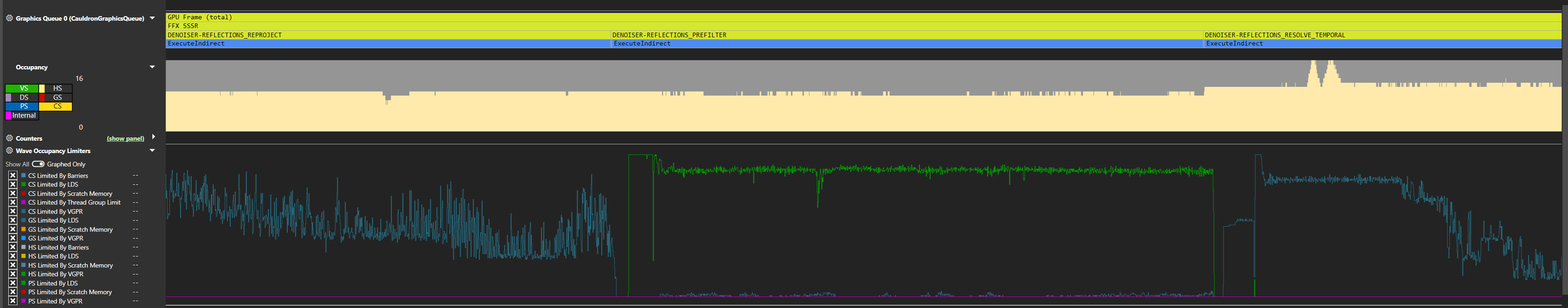
The theoretical occupancy or maximum achievable occupancy is only an upper bound of what we’ll call now the measured occupancy. RGP is a great tool to explore the measured occupancy and we will be using its dedicated wavefront occupancy tab for this next section. In this view, the top graph plots the measured occupancy, and the bottom bar chart shows how the different draws and compute dispatches overlap on the GPU. From now on, we’ll use the term “work item” to talk about them both. To get more information on a specific work item, just select it from the bottom bar chart and look at the details panel on the right hand side.

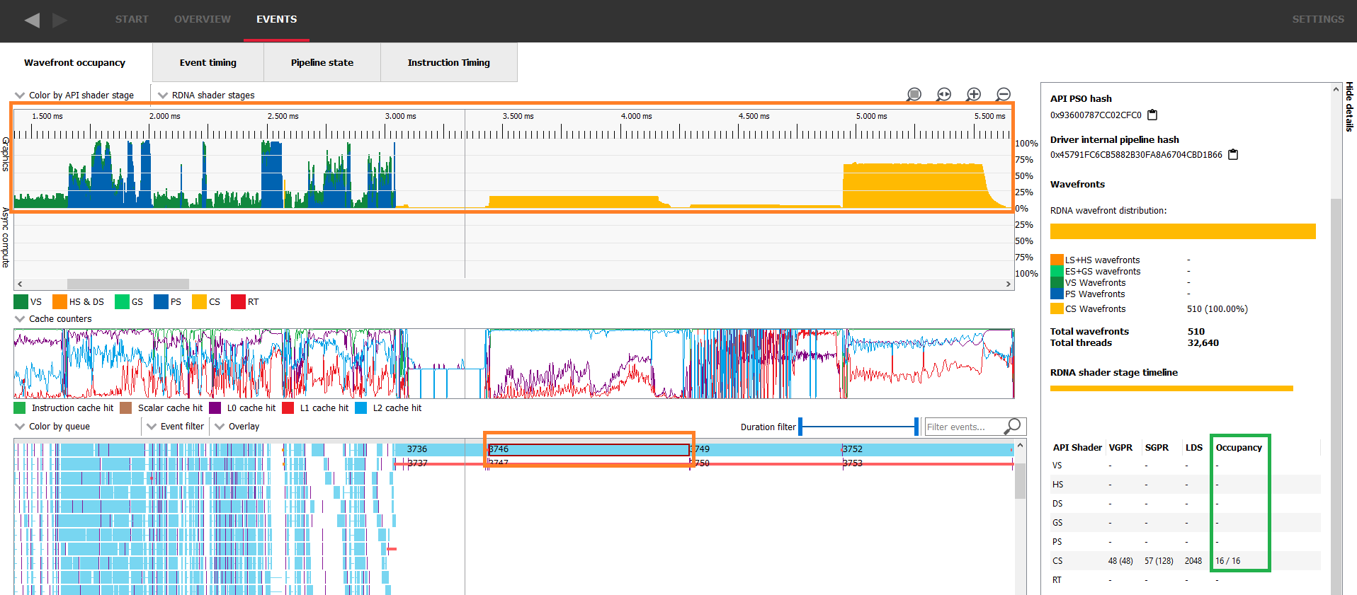
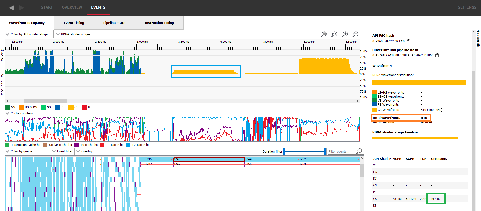
The occupancy column of the details panel shows the theoretical occupancy for this specific work item. In this capture we can immediately see that the measured occupancy is not constant and does not necessarily match the theoretical occupancy. In the following image, the measured occupancy graph lies within the blue rectangle, the selected work item is in the orange rectangle and the green one shows where to look for theoretical occupancy in the details panel.

There are mainly two reasons why the measured occupancy can’t reach the theoretical occupancy, either there is not enough work to fill all the slots or the GPU is not able to launch those wavefronts quickly enough.

Lack of work limited occupancy

An AMD Radeon™ RX 7900 XTX has 6 Shader Engines (SEs), 8 Work Group Processors (WGPs) per SE, and 4 SIMDs per WGP. This gives you a total of 6 * 8 * 4 = 192 SIMDs. So any workload short of 192 * 16 = 3072 wavefronts (remember there are 16 wavefront slots per SIMD) will never be able to reach 100% occupancy, even if the wavefronts are never resource limited. This scenario is usually pretty rare and fairly easy to detect.

The execution of such a small workload will be very quick on the GPU and the details panel will display how many wavefronts were assigned in total. In the following image, the selected work item’s theoretical occupancy is 16/16 as shown in green in the details panel, yet the measured occupancy doesn’t even reach 4/16 as shown in blue. This is because there are only 510 wavefronts in flight as shown in orange in the details panel.

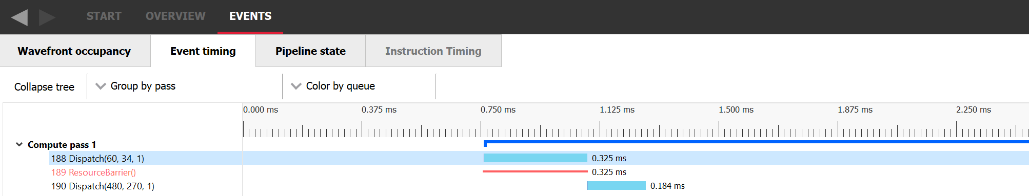
Another classic scenario where there aren’t enough waves in flight to fill the GPU is at the end of the execution of a workload when most of the work is done and only a few remaining wavefronts need to be executed. In the following image, we can see in the blue rectangle that dispatch 188 starts ramping down a bit before 1.05ms and doesn’t remain at its full occupancy for the whole duration of its execution. As soon as all the threads of dispatch 188 are retired, dispatch 190 starts. This happens because event 189 is a barrier preventing the two dispatches from overlapping.

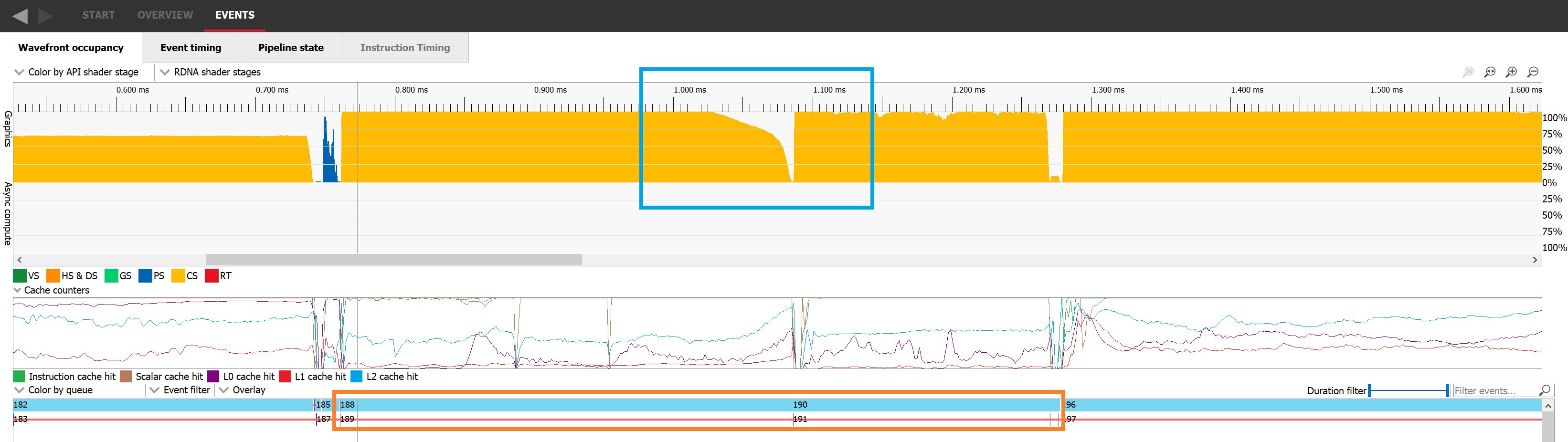
If we switch to the Event timing tab, we can look at the events in a more sequential order. Dispatch 188 was issued, then a resource barrier was issued which prevents overlap with the next work item, and finally dispatch 190 was issued.

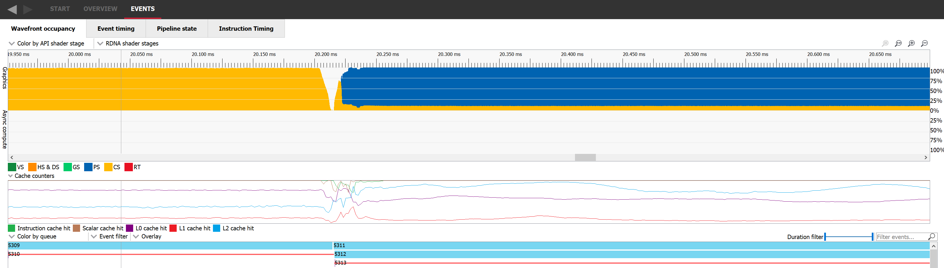
The way to improve occupancy for both of those scenarios is to find a way to overlap work. If we can manage to make two occupancy-limited workloads execute in parallel, it’s likely the overall occupancy of the GPU will increase. To make this happen, we need to pick two workloads that don’t have any dependencies with one another and issue them to a command list without any barrier between them. In the following picture we can see dispatch 5311 where occupancy is represented in yellow nicely overlapping with draw 5312 where occupancy is represented in blue. Sadly, this is not always possible.

Launch rate limited occupancy

Figuring out when the occupancy is limited by the GPU not being able to launch waves fast enough is a bit trickier. The most obvious place is when two workloads have a dependency. The GPU needs to drain the first workload before the second one can start. Once the second starts from an empty GPU, the measured occupancy rises as the GPU ramps up on work. This usually only lasts for a really short period of time and is unavoidable. In this case again, the only solution would be to remove the dependency and make the two workloads overlap as we described in the previous paragraph.

However, the same thing can happen in the middle of the execution of certain workloads if the waves for that workload execute faster than the GPU can launch them. This is not ideal and the occupancy will be limited by the rate at which the GPU can launch waves. Launching a new wave is a more complex operation than simply assigning it to a SIMD so it can run. Work has to be done to setup the contents of various registers so that execution can start, and each shader type has particular requirements.

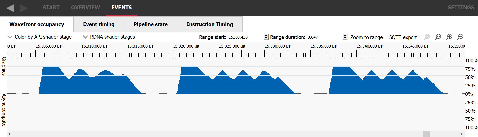
The easiest way to detect a launch rate limited occupancy in a RGP capture is to look for a workload that started with a really high occupancy, which then decreased and never caught that peak occupancy again. It will often oscillate before stabilizing to its average value. At the beginning of such workloads, many waves are launched on the GPU but then stall waiting for some initial data to be made available. Once the data required to execute the waves is at least partially cached, they execute faster than the GPU can start more, making the occupancy decrease, and so on.

For a pixel shader, if none of the previously described situations seem to match your workload, it’s possible that the GPU is running out of LDS to store the interpolants sent from the VS to the PS. Unfortunately, the amount of LDS required for a PS cannot be evaluated at compile time. It depends on how many unique primitives a single wavefront is dealing with which is evaluated at runtime. In this case, one should investigate what kind of geometry is being rendered. If a lot of tiny triangles are being drawn, it’s likely that each wavefront will end up dealing with multiple primitives. One way to mitigate this issue to tune your game’s level of detail (LOD) system.

Occupancy limiters

In the previous paragraphs, we tried to give an understanding of what the occupancy limiters are and why. However, when investigating occupancy in practice it might be easier to have a tool identify for you which parts of the frame are occupancy limited and by which limiting resource. This is exactly what the “WaveOccupancyLimiters” provides, as exposed by the AMD plugin for Microsoft® PIX. You can request those directly in the bottom part of the overview tab.

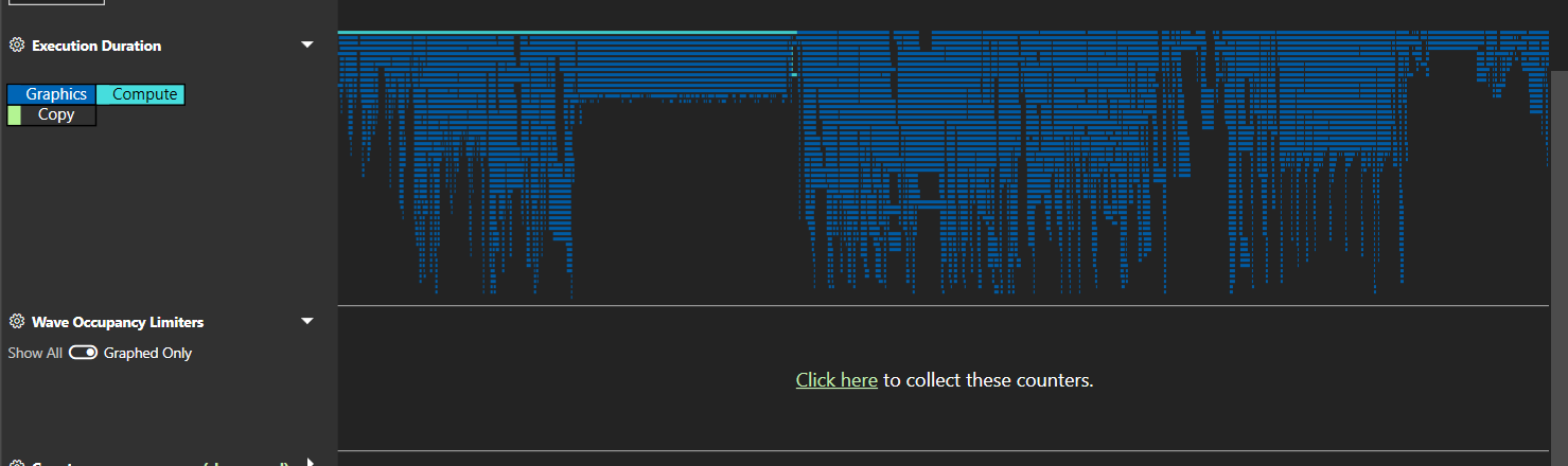
Once the counters are captured, PIX will plot them against time just like the other counters.

Limiters list

If we look at the list of counters, we can see that even though they are specialized by wave type, they can mostly be split into 4 categories.

Limited by VGPR
Limited by LDS
Limited by Thread Group Size
Limited by Barriers

The first three ones we’ve seen before. In order to launch wavefronts on a SIMD, the scheduler needs to reserve all the required execution resources they might need in advance, including VGPRs and LDS. In the case of a compute shader, there must be enough of these resources for the entire threadgroup. Because you define the size of that threadgroup, you can influence this resource requirement.

As for barriers, the GPU can track up to 16 barriers in flight per pair of SIMDs. As a reminder, each SIMD can have 16 waves assigned, for a total of 32 waves per SIMD pair. When running compute shaders, the resources required to run an entire threadgroup will be allocated and deallocated together, which means the GPU needs to be able to synchronize the waves that make up a threadgroup at the end of their execution. This synchronisation requires a barrier and it is thus possible to use up all the barrier resources in a worst case scenario.

A barrier is only required if a threadgroup is made of at least 2 waves. So we can at most have 32 / 2 = 16 threadgroups that require a barrier. This is perfect since we have 16 barrier resources. However, if 1 wave finishes, it frees a slot on the SIMD but it can’t free its needed execution resources because it has to wait for the 2nd wave of its threadgroup to finish too. Since a wave slot is now available but cannot be filled, we are occupancy limited. In this scenario we are Thread Group Size limited because we need 2 wave slots to assign a single threadgroup.

Now, if the second wave of that threadgroup finishes, we’re not occupancy limited anymore. The slots, the resources and the barriers required for this entire threadgroup will be freed. However, if a wavefront from a different threadgroup finishes, we now have 2 slots available, potentially enough resources to run another threadgroup but no barrier available to launch it. In this case we are occupancy limited by barrier resources. This is a very specific case and in practice it will be super rare.

Reading the limiters graph

Because PIX plots these counters over time and displays the value of the counter as a percentage, it is natural to think that the lower the percentage the less occupancy bound the shader is. Sadly, this is not true at all. Those counters should mostly be used as a binary metric to figure out which resource is limiting the occupancy. To understand why that is, we need to understand how those are gathered. Every clock, if there are wave slots available, the scheduler will try to launch new waves. If that is not possible, the relevant occupancy limiter counters will be incremented. This will happen every clock as long as a wave slot is available and the GPU is not able to schedule a new wave. At the end of the workload, we’ll divide those counters by the number of total clocks the workload took to figure out what percentage of that workload was actually bound by those limiters.

The important thing to understand is that no matter what that percentage is, it doesn’t say anything about occupancy. Whether a workload that is running at a particular occupancy is limited has no impact on its ability to hide latency. All that matters is whether there’s enough occupancy to hide any latency. The limiter percentages will vary based on how long it takes for the waves to execute. If the waves are long-running, the scheduler will likely not often find any new waves to launch and thus count many clocks for that limiter. On the other hand, if the waves are very short, there are often new slots available and so the GPU less often fails to launch new waves. The limiters percentage can give us some idea of the way the GPU launches waves but it will not give any extra information on occupancy. If one of the counters is greater than 0, then it’s a limiter and that’s all we can infer from it.

Peak occupancy does not always mean peak performance

Before we move on to the practical implications of understanding GPU occupancy, it’s worth understanding one of the most important practical aspects of occupancy that you might encounter when you’re profiling and trying to optimise the performance of your shaders. We’ve discussed what intra-WGP shared resources can limit occupancy, which can give you the intuition that your job as the shader programmer is to maximise occupancy by limiting the usage of those shared resources.

However, there are also shared – and often scarce! – resources outside of the WGP in the rest of the GPU that your shaders make heavy use of when it comes to memory. Each external memory access has to pass through the GPU’s cache hierarchy, hopefully being serviced by the caches along the way so that it saves precious memory bandwidth and reduces execution latency. In any modern GPU there are multiple levels of that hierarchy for each access to pass through.

Because wavefronts from the same shader program tend to run together, doing roughly the same thing at roughly the same time, whenever they access memory they’ll tend to do so in groups. Depending on the shape of memory access being performed and the amount of data that is being written from or read into the shader, it’s possible to thrash the caches in the hierarchy.

So occupancy going up can mean performance goes down, because of that complex interplay between getting the most out of the GPU’s execution resources while balancing its ability to service memory requests and absorb them well inside its cache hierarchy. It’s such a difficult thing to influence and balance as the GPU programmer, especially on PC where the problem space spans many GPUs from many vendors, and where the choices the shader compiler stack makes to compile your shader can change between driver updates.

Practical implications

In this last section we wanted to concentrate all the knowledge we have tried to convey in this post to a format that can be more easily parsed if one were to visit this post again. We’ll first answer a few classic questions about occupancy and then provide a small guide on how to tackle improving occupancy for a given workload.

Q&A

Q: Does better occupancy mean better performance?
A: No, it will only improve performance if the GPU can use the occupancy to hide latency while balancing the available performance of the cache hierarchy.

Q: When should I care about occupancy?
A: Primarily when a workload is sensitive to memory performance in some way.

Q: Does maximum occupancy mean that all the memory access latency from my shader is hidden?
A: No, it only means that the GPU maximises its capacity to hide it.

Q: Is lower theoretical occupancy always bad for performance?
A: Just as maximum occupancy can hurt performance, lower occupancy can help it, but always profile and always check that low occupancy shaders are not spilling registers to memory (see the last paragraph below).

How to improve occupancy

If your theoretical occupancy is low and your measured occupancy matches it, try improving the theoretical occupancy with the following recommandations. Otherwise, skip to 2.
- Find the most limiting resource amongst VGPR and LDS and try to use less of those.
  - Remember that a bigger wave size implies more resources per wave and thus less resource allocation granularity.
  - While it is possible to ask for a specific wave size in Shader Model 6.6, please remember that it does not just affect the potential occupancy of a shader and should be used incredibly carefully. The full effects of such a change are complex and outside of the scope of this post, and it’s very difficult for wave size choices to be performance portable.
- For compute shaders, make sure the threadgroup size is not the limiting factor.
  - If it is, try reducing its size to improve the granularity of the scheduling. For more information about the impacts of threadgroup size, please read the following GPUOpen article: Optimizing GPU occupancy resource usage with large thread groups.
If your theoretical occupancy is decently high but your measured occupancy doesn’t match it, investigate the following points
- Make sure that your workload generates enough wavefronts to fill the GPU.
  - If not, the only solution is to overlap some other workload with it.
- If your workload generates enough waves, make sure each wave has enough work to do to offset the cost of launching the wave.
  - For compute shaders, try making each wavefront do more work by batching work items together.
  - For fragment shaders, try reducing the number of interpolants sent from the VS to the PS to see if that helps.
- If none of the above applies and you’re optimizing a pixel shader, the GPU might be running out of LDS to store the interpolants. The amount of required LDS is heavily influenced by the number of primitives a SIMD is dealing with.
  - If your geometry is made of a lot of tiny triangles, try improving your level of detail (LOD) system.

Side note: register spilling

When we described theoretical occupancy, we first explained how it is tied to the amount of resources required by a wavefront to be executed. We also mentioned that a wavefront cannot be launched if there aren’t enough resources available for it, but that’s not strictly true when it comes to VGPR usage: the shader compiler has a mechanism in place that lets it “spill” registers to memory.

This means that instead of requiring the shader to use a huge amount of registers, it can decide to reduce that number and place some of those in memory instead. Accessing the data stored in memory has a much greater latency than accessing the data stored in physical registers and this usually greatly impacts the performance. While this is not strictly speaking related to occupancy, when a shader has a low theoretical occupancy and is limited by GPR pressure, it is worth checking whether it is spilling or not. The pipeline tab of RGP will let you know for a given work item if the shader compiler had to spill registers to memory.

I would like to thank Pierre-Yves Boers, Adam Sawicki, Rys Sommefeldt, Gareth Thomas, and Sébastien Vince for reviewing this post and providing invaluable feedback.