AMD FidelityFX™ Variable Shading
AMD FidelityFX Variable Shading drives Variable Rate Shading into your game.
In this article, we start this series by motivating the evolution from a vertex-shader based pipeline towards mesh shading.
To appreciate the flexibility and potential performance gains of the mesh shader pipeline, it might be helpful to look at how the GPU processes traditional draw calls using a combination of vertex and index buffers.
For traditional graphics pipelines, a mesh is commonly defined as a set of vertices with each triplet of consecutive vertices forming a triangle. To reduce data duplication, an optional index buffer can be used to define triangles as a set of three indices, with each index referencing a different vertex. For the purpose of comparing mesh shaders to the vertex pipeline, we will only focus on the latter indexed vertex shading.
As an example, we will use the following index and vertex buffer and follow the first four triangles through the GPU to the rasterizer.

Before these primitives can be rasterized and shaded, they pass through the Input Assembler and a programmable geometry pipeline comprised of up to four different shaders.
A vertex shader is required in every geometry pipeline.

For simplicity, in this first blog post, we will only look at how vertex shaders map to our RDNA™ hardware. The geometry and tessellation shader stages will be covered in a later blog post.
For each vertex that is referenced by an index buffer, the GPU needs to run a vertex shader instance to transform the vertex from its input layout of the vertex buffer(s) to a position in clip-space. As the input mesh uses an index buffer, the same benefits of reusing vertices should also apply here and reduce the overall number of potentially costly vertex shading operations. The input assembler is responsible for resolving the index buffer and for initiating the subsequent processing of vertices.
An obvious way of implementing vertex reuse in the input assembler would be to run a vertex shader instance for every vertex in the vertex buffer and store the transformed vertex.
This approach, however, is not feasible to implement, as storing potentially millions of transformed vertices might exceed the memory capacity of the GPU.
Additionally, such an implementation would delay the primitive assembly and thus shading operations until all vertex shader instances have finished executing.
So instead, we need a system that can shade batches of vertices in parallel and assemble already shaded vertices into primitives, whilst other vertices are still in flight or even unprocessed.
On RDNA™ graphics cards, this is implemented using our Next Generation Geometry (NGG) technology, which we will look at in the next section.
To illustrate the various components of the NGG pipeline and how they work together, we will follow an exemplary indexed draw call through the geometry processing stage. As before, for simplicity, the draw call only uses a vertex shader and no geometry or tessellation shaders.
To draw our example mesh, we submit the following draw call to a graphics command list.
graphicsCommandList->DrawIndexedInstanced(12 /* index count */, 1 /* instance count */, 0 /* start index location */, 0 /* base vertex location */, 0 /* base instance location */);Once the command buffer is submitted and the draw call is processed by the API runtime and the GPU driver, a draw command is sent to the GPU. This command is received and processed by the following components:

To determine, which vertices need to be processed by a vertex shader, the geometry engine selects a subset of primitives from the index buffer. For demonstration purposes, the geometry engine chooses four triangles from our example mesh above. This subset of triangles forms a primitive subgroup: To build a primitive subgroup, the geometry engine scans the indices of triangles of a subset and creates a list of unique vertex indices. Then, the geometry engine reindexes the vertex indices from the index buffer with respect to the unique vertices list of said subgroup. Conceptually, a primitive subgroup, i.e., the pair of reindexed vertex indices and the unique vertices, forms a small mesh - or meshlet - with its own set of vertices and indices. As these indices do not directly reference vertices in the original input vertex buffer, but rather reference vertex indices in the unique vertex list, we will refer to these indices as primitive connectivity.

The vertices in a primitive group will be processed together and once vertex processing is complete, the primitive connectivity is used to assemble them into triangles ready for rasterization. After a primitive group is formed and sent off for processing, the geometry engine repeats the same process for the next subset of primitives in the index buffer, until all primitives have been rendered.
As illustrated above, primitive connectivity indices can only reference vertices within the same primitive subgroup and thus the shaded vertices are only reused within the primitive subgroup.
What does all of this mean for vertex invocations and vertex reuse?
In order to maximize the vertex reuse, we ideally want to have all primitives that reference a vertex in the same primitive subgroup. In other words, we want each vertex to exist in only one primitive subgroup. Otherwise the GPU will invoke the vertex shader multiple times for the same vertex, thereby performing redundant calculations and degrading overall performance. As primitive subgroups are bound by either a maximum number of vertices or a maximum number of primitives, an ideal vertex reuse, i.e., each vertex is only processed once, is not possible, in general.
Instead, so called vertex cache optimization aims to decrease vertex duplication to an acceptable level. Though primitive subgroups are computed and rasterized independently from each other, and thus differ from a traditional vertex cache that stores transformed vertices ready for reuse on following triangles, the term vertex caching is still often used to describe the primitive subgroup behavior. Libraries such as zeux’ meshoptimizer try to approximate the GPU’s vertex caching behavior and reorder the index buffer accordingly. Primitives sharing the same vertex become clustered together, thus increasing the chances of finding the vertex in a vertex cache or bundling all these primitives in the same primitive subgroup. This pre-processing can and should be applied statically to any triangle mesh.
As an example, the Stanford Bunny is a photo-scanned mesh with almost 70 thousand triangles and almost 35 thousand vertices.
Due to its photo-scanned nature, vertices are organized in a grid-like fashion and triangles are organized as vertical lines in this grid.
These lines cause vertices in a subgroup to be reused at most twice, which causes vertices to be shaded multiple times.
Using zeux’ meshoptimizer and the meshopt_optimizeVertexCache function greatly reduces duplicate vertex shading and thereby improves performance.
| Mesh | Optimized Mesh | |
|---|---|---|
| Vertices | 34.8k | 34.8k |
| Vertex Shader Invocations | 143.9k | 48.9k |
| Duplication Factor | 4.13 | 1.40 |
| Visualization: Different colors represent different primitive subgroups. | 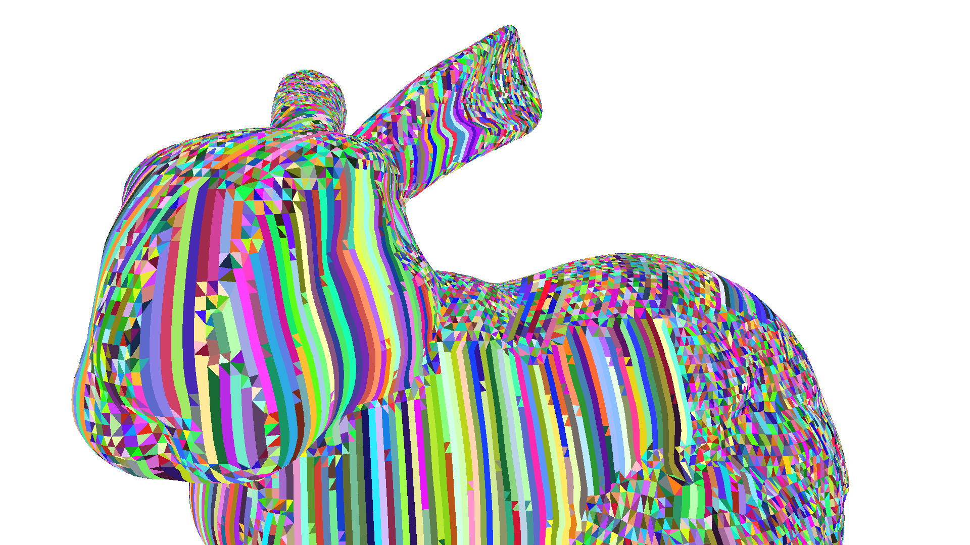 | 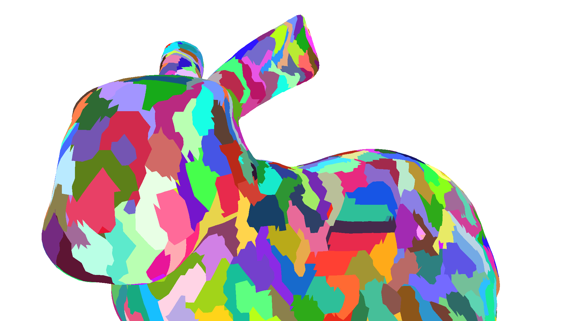 |
So far, we have covered how the geometry engine generates primitive subgroups from the incoming vertex and index buffer(s), but not how primitive subgroups are processed and rasterized. Instead of the typical vertex, geometry, and programmable tessellation shader stages, NGG combines different functionalities of each stage into two different shaders:
As the name suggests, primitive shaders are used to process primitive subgroups.
Each thread of the primitive shader gets assigned to one vertex index and one primitive of the primitive group.
A primitive shader thread receives the primitive connectivity information of its assigned primitive and loads the vertex information of its assigned vertex from the respetive vertex buffer(s).
Then, it carries out vertex shading.
Finally, the primitive shader issues the exp instruction to export both the received primitive connectivity information and the transformed vertex to the shader export, ready for primitive assembly and rasterization.
As primitive shaders can also modify the primitive connectivity information, they can also be used to implement both tessellation domain and geometry shaders.

The primitive assembler loads primitive connectivity data for a primitive along with the three referenced vertices, assembles the triangles, and performs culling as well as view transform operations before sending the primitive to the rasterizer and thus concluding our trip down the NGG pipeline.
Summing up, we have seen how an RDNA™ GPU handles indexed draw calls and how the Next Generation Geometry pipeline handles vertex reuse. However, an indexed vertex pipeline still poses challenges and limitations. The vertex pipeline does not offer any direct control over vertex shader invocation and vertex reuse. The limited control through vertex cache optimization is often challenging to implement. Vertex cache optimizers aim to support a wide variety of hardware vendors and hardware generations and therefore do not yield a solution performing equally well on all GPUs. Lastly, index buffers have to adhere to fixed formats that can be understood by the GPU, which limits the flexibility for implementing indexed based decompression techniques.
In the next chapter, we are going to look at how mesh shaders address the aforementioned challenges and limitations, which further possibilities are introduced by mesh shaders, and how mesh shaders fit within the NGG pipeline.
Mesh shaders were introduced to Microsoft DirectX® 12 in 20191 and to Vulkan as the VK_EXT_mesh_shader extension in 2022.
Mesh shaders introduce a new, compute-like geometry pipeline, that enables developers to directly send batches of vertices and primitives to the rasterizer.
These batches are often referred to as meshlets and consist of a small number of vertices and a list of triangles, which reference the vertices.
Conceptually these meshlets are very similar to the primitive subgroups we explored earlier in that they can also be used to represent a small part of a larger mesh, but as these meshlets are completely user-defined, they can also be used to render procedural geometry such as terrains or tessellated geometry such as subdivision surfaces.
The latter will be covered in more detail in a later entry to this blog post series.
In this first installment, we will focus on rendering a triangle mesh using mesh shaders.
Mesh shaders introduce two new API shader stages:
These two new shader stages replace the traditional geometry pipeline of vertex-, hull-, domain-, and geometry-shader and cannot be combined with any of these stages.

Both mesh- and amplification shaders employ a programming model that closely matches the programming model of compute shaders and is thus more inline with the modern graphics card architecture of unified compute hardware. Instead of having one thread per vertex, sample, or primitive with no visibility or communication to other threads, mesh shaders are organized in thread groups. Each thread group specifies and then writes a variable number of vertices and primitives, with no requirements to tie primitives or vertices to specific threads. Any thread can write any vertex or primitive, though some general best practices, which we will discuss in the next blog post, should be kept in mind.
With the compute-like organization in thread groups, launching mesh shaders also differs from traditional draw calls.
Instead of specifying number of vertices or indices to process, the DispatchMesh (Vulkan: vkCmdDrawMeshTasksEXT) command specifies the number of mesh shader thread groups to launch in the same three-dimensional grid as compute shaders.
graphicsCommandList->DispatchMesh(threadGroupCountX, threadGroupCountY, threadGroupCountZ);This direct launch of thread groups also means that mesh shaders skip the input assembler stage. This gives developers complete control over which primitives to export from a mesh shader and removes any limitations on the input data. Like a compute shader, a mesh shader can read from and even write to any resource. The direct control over which primitives to rasterize also enables the possibility for culling individual primitives or - in combination with an amplification shader - entire meshlets.
Bypassing the input assembler necessitates off-loading vertex reuse computation into a pre-process. This avoids re-computing the reuse information every frame or draw-call over and over again. Instead it can be shared across multiple draw calls and frames. Removing the input assembler also means that it cannot become a pipeline bottleneck. This allows mesh shaders to directly scale with different GPU configurations. Additionally, retiring the legacy geometry amplification programming models of tessellation and geometry shaders means geometry amplifications in mesh shaders can better map to compute hardware and alleviates the use of fixed function hardware.
Lastly, the organization of mesh shaders in thread groups allows the threads to communicate via wave intrinsics and group shared memory to cooperatively compute one or more vertices or primitives.
In summary, the compute-like programming model of mesh shaders enables developers to overcome key limitations of the traditional vertex pipeline, whilst also enabling greater flexibility for advanced rendering techniques, such as triangle culling or real-time geometry decompression. As a case study on actual mesh shader applications, we will look at geometry decompression in a later blog post.
Before taking a look at amplification shaders, we briefly look at how mesh shader fit into the NGG pipeline.
As discussed in the first section, the NGG pipeline consists of two shader stages, the surface shader and the primitive shader. Primitive shaders are used to process primitive groups and are able to export both vertex attributes as well as primitive connectivity information - i.e., primitives - to the primitive assembler via the shader export. It is easy to see how this functionality can be directly used to map mesh shaders onto the NGG pipeline.
The DispatchMesh command directly specifies a three-dimensional grid of mesh shader thread groups to be launched, which in turn directly map to primitive groups.
Thus no vertex de-duplication or reuse scanning is needed before launching a mesh shader thread group.
We discussed previously that mesh shader launches are thus quite similar to compute shader dispatches.
However, mesh shader thread groups are still launched through the geometry engine.
The geometry engines in this case is still responsible for tracking and managing allocations in the shader export and managing the state of the primitive assembler (primitive mode, culling, etc.).
Most importantly, as the number of vertices and primitives are not known before launching a mesh shader, the geometry engine receives the actual vertex and primitive count and forwards it to the primitive assembler.

As the duties of the geometry engine when using mesh shaders differs vastly from those of traditional vertex shading, the geometry engine implements a special fast launch mode, which bypasses any vertex reuse checking and primitive subgroup formation stages.
Amplification Shaders are an optional shader stage that is run before the mesh shader and can control the subsequent launches of mesh shader thread groups. Each amplification shader thread group can launch a variable amount of mesh shader thread groups, i.e., - as the name implies - amplify the overall workload that is executed on the GPU. This amplification, however, is different from the one achievable by using tessellation shaders. Instead of amplifying the number of primitives inside a control patch through fixed-function hardware, amplification shaders operate on a coarser level and only specify the number of mesh shader thread groups to launch. That said, it is possible to mimic the effects of the fixed function tessellation amplification using amplification shaders.
In order to launch mesh shaders, amplification shader can call the DispatchMesh shader intrinsic and specify a three-dimensional grid of mesh shader thread groups to launch.
This intrinsic behaves in the same way as the DispatchMesh command on the CPU.
Whereas the CPU can write to or modify the shader’s root signature in between DispatchMesh calls, the amplification shader cannot.
Instead amplification shaders can pass a user-defined payload from the amplification shader to all subsequently launched mesh shaders.
DispatchMesh(threadGroupCountX, threadGroupCountY, threadGroupCountZ, payload);Launching amplification shaders from the CPU is done in the same way as launching mesh shaders: If a graphics pipeline state specifies an amplification shader, the three-dimensional grid specified in the DispatchMesh command directly refers to the grid of amplification shaders to launch.
Selecting whether to launch mesh- or amplification shaders is not possible and requires separate graphics pipeline states.

This direct work amplification on the GPU may seem similar to the recently introduced GPU Work Graphs, but some key differences and limitations apply to amplification shaders:
DispatchMesh intrinsic inside an amplification shader only accepts a single payload for all subsequently launched mesh shader thread groups.
Similarly, an amplification shader thread group can only call DispatchMesh once.Even with these limitations, amplification shaders extend the flexibility of the mesh shader pipeline by allowing for dynamic work amplification or work reduction entirely on the GPU. Examples of applications of amplifications shaders include:
In the case of instance culling and dynamic LODs, the number of mesh shader thread groups that each thread of an amplification shader thread group wants to launch will vary across the thread group. This can slightly complicate the assignment of mesh shader thread groups to specific elements in the payload.
We will cover meshlet culling for meshes and dynamic level-of-detail for subdivided geometries in more detail in a later blog post.
To summarize what we have explored so far: We have seen how RDNA™ GPUs handle indexed geometry and how regular geometry is rendered in primitive subgroups - or meshlets - and the challenges that come along with it, such as vertex cache optimization. We have seen how mesh shaders overcome these challenges by offering developers full control over the geometry processing pipeline, thus alleviating the need for any runtime vertex reuse checking while at the same time allowing for more flexibility in geometry processing. We looked at how mesh shaders map to the Next Generation Geometry pipeline and how the mesh shader fast launch path works. We also covered amplification shaders and touched on their capabilities to enable a dynamic GPU-only rendering pipeline.
In the next installment of this blog post series, we will discuss some best practices for writing mesh shaders and cover profiling and optimizing mesh shaders. In further blog posts, we show case-studies of using mesh shaders and explore their various features. In particular, we will be looking at geometry decompression and procedural geometry.
Links to third-party sites are provided for convenience and unless explicitly stated, AMD is not responsible for the contents of such linked sites, and no endorsement is implied. GD-98
Microsoft is a registered trademark of Microsoft Corporation in the US and/or other countries. Other product names used in this publication are for identification purposes only and may be trademarks of their respective owners.
DirectX is a registered trademark of Microsoft Corporation in the US and/or other countries.