AMD FidelityFX™ Variable Shading
AMD FidelityFX Variable Shading drives Variable Rate Shading into your game.
March 2024 update for release of Microsoft® Work Graphs 1.0: Use this latest AMD driver.
In this article we’re going to practice using the Workgraph API, published by Microsoft earlier. If you’re unfamiliar with the basic syntax of Workgraphs, there is a great introduction here on GPUOpen, which I recommend reading GPU Work Graphs Intro.
Workgraphs are exceptionally good at expressing pipelines. If you think about implementing an algorithm on the GPU, you probably often approach it as one monolithic program run on as many GPU work units as possible. After all, splitting an algorithm into multiple phases with the current language and API has very little upside:
Whatever opportunity in workload reduction and shaping that is created by phasing an algorithm, needs to be worth more than the disadvantages caused by it.
The Workgraphs API is not just providing a syntax to express pipelines and graphs, it solves the aforementioned problems under the hood as well:
In this part of the series we’re going to pick a small sample algorithm, show the workload reducing and shaping opportunities arising from breaking it into stages and how Workgraphs can maximize performance inherit therein.
The small sample algorithm we’ve chosen for demonstration is a scanline rasterizer. To keep the scope simple, we picked a algorithm variation which gracefully deals with the edge case of near plane intersections and needs no triangle clipper. Furthermore this sample isn’t meant to be an industrial strength copy’n’paste template, it’s to teach about Workgraphs and many things unrelated to Workgraphs have been left to be solved, like edge tie-breaking and some precision inaccuracies or hierarchical-Z testing: Triangle Scan Conversion using 2D Homogeneous Coordinates
The algorithm can be described simplified with these steps:
It’s a small algorithm (~100 lines of code), that solves the problem of triangle rasterization well. We will simply refer to this algorithm as the rasterizer onwards, and if we say bounding box it means a screen space AABB.
In the following, we design the algorithm, then we go into the implementation details, and finally we’ll see some results. In your own projects there’ll be quite some back and forth between experimentation and consideration. But one good aspect of the new Workgraphs paradigm is that this feels very comfortable to do. Once you have a stable interface between the application and the shader program, you can mostly stay in the shader code and try different approaches.
Let’s transform the rasterizer algorithm step by step towards an implementation which works well on a GPU and takes advantage of the capabilities of Workgraphs. Naturally we’re going to break the algorithm into smaller pieces, taking advantage of routing data between the algorithm stages freely, and cull redundant data away.
A GPU is currently practically a SIMD processor. The width of the SIMD vector varies between implementations and is commonly between 16 and 64 lanes wide.
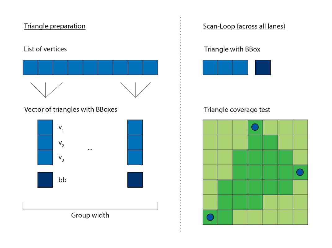
The rasterizer can be vectorized easily. Each lane is responsible to process a different triangle. The scan loop needs to iterate for as long as a participating triangle use it’s parameters. For example, if there’s two triangles with respective bounding boxes of 48x6 and a 8x92, then the loop needs to iterate over the range of 48x92 to cover the area of both simultaneously:

This is rather inefficient, as almost all of the area union is empty and not useful to either triangle. It’s better to reduce the dimensionality of the shared loop from 2D to 1D. The two example triangle’s loop parameters become 288 and 736 respectively, which is much better than the prior resulting 4140 iterations:
float BBStrideX = (BBMax.x - BBMin.x + 1);float BBStrideY = (BBMax.y - BBMin.y + 1);float BBCoverArea = BBStrideY * BBStrideX - 1.0f;
float y = BBMin.y;float x = BBMin.x;
while (BBCoverArea >= 0.0f){ x += 1.0f; y += x > BBMax.x; if (x > BBMax.x) x = BBMin.x;
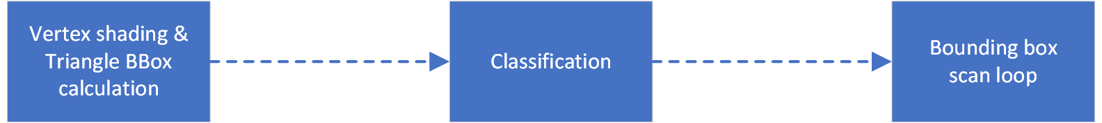
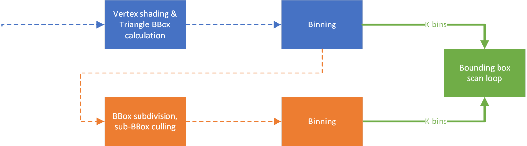
BBCoverArea -= 1.0f;While the first step is already a good improvement, it would be nice if we could improve it further still. Can we make it happen that the triangle’s areas are similar to each other? It would allow the participants of the shared loop over the SIMD vector to be more coherent, and we don’t encounter situations where a small triangle is processed together with a big triangle. For this we have to break the rasterizer into two phases:
Between these two phases, we can now look at all of the triangles, group them by area and launch the loops with triangles which are of similar size. Normally this would cause significant overhead (programming and executing) in the regular Compute API, but with the Workgraphs API this is fairly straightforward, as we can divert the output of the first phase into a collection of second phases.
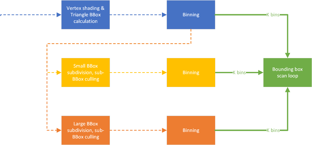
There remains a problematic detail, that is that triangles can have areas anywhere between 1 and the entire screen (~8 million for 4k). We don’t want to specify that many variations of the scan loop. Additionally the frequencies of triangle sizes fall off fairly fast for a real world scene, and you’d be pressed to find more than a couple of triangles occupying the large areas. Instead we can bin the triangles into a more manageable set of area properties. For generality we should not base this on specific triangle frequencies, but rather choose an expected distribution. A logarithm is a good choice, and base 2 is computable very quick (maybe you spot the connection to information entropy).
// Calculate rasterization area and binfloat2 BBSize = max(BBMax - BBMin + float2(1.0f, 1.0f), float2(0.0f, 0.0f));float BBArea = BBSize.x * BBSize.y;int BBBin = int(ceil(log2(BBArea)));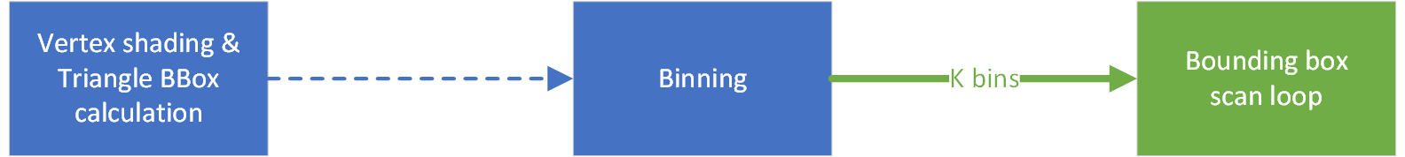
To support 4k we’d have to provide 23 rasterization loops: 22.93 = log2(~8mil.), although even with applying the logarithm there are going to be very few triangles in the last bins. Additionally, for generality, we wouldn’t like a limit on the triangle’s sizes anyhow. And as one additional worry: a shader program running a loop for 8mil. iterations is extremely inefficient on a parallel processor like the GPU. What we can do instead, is breaking up larger areas into smaller areas. And this sounds familiar, this is what the hardware rasterizer also does, it subdivides screen space into fixed sized tiles, and if a large triangle is processed it distributes the same triangle to that many tiles. It allows the hardware to parallelize triangle rasterization at a modest cost. The idea provides us with three benefits:
There is one more indirect benefit emerging, if we look for optimization opportunities, which is that we don’t need to rasterize empty bounding boxes. Once we chop up the original triangle’s bounding box into smaller ones, some of the smaller bounding boxes now might reside entirely out of the original triangle’s area. A box is a rather poor approximation for a triangle: essentially half of the box’s area is empty space. If our maximally binneable area is small compared to the incoming area, then we can cull a large amount of iterations which don’t do anything except failing to qualify for the triangle’s interior:
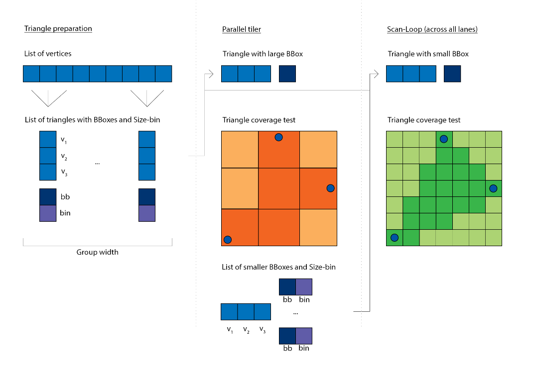
This, again, can be parallelized by passing the subdivision factors directly to a Dispatch, much the same as what the hardware does.
Now we come to our first Workgraphs API specific optimization. You can launch a Broadcasting node with dynamic Dispatch parameters:
struct SplitRecord{ uint3 DispatchGrid : SV_DispatchGrid;and
[Shader("node")][NodeLaunch("broadcasting")][NodeMaxDispatchGrid(240, 135, 1)] // Enough of a limit to allow practically unlimited sized triangles[NumThreads(SPLITR_NUM_THREADS, 1, 1)]void SplitDynamic(or you can used fixed Dispatch parameters:
[Shader("node")][NodeLaunch("broadcasting")][NodeDispatchGrid(1, 1, 1)] // Fixed size of exactly 1 work group[NumThreads(SPLITR_NUM_THREADS, 1, 1)]void SplitFixed(The fixed Dispatch parameter variation is much easier to optimize by the scheduler than the dynamic Dispatch variation. Consider we’re launching 2x Dispatches X,1,1 and X,1,1 and we don’t use Y and Z as in the following “uint WorkIndex : SV_DispatchThreadID”.
For a regular Compute Dispatch and for a Workgraphs dynamic Dispatch this are unknown and variable Xs, and the scheduler together with the allocator need to prepare for these unknowns. But a Workgraphs fixed Dispatch knows it’s X is always the same, and it knows you’re not using Y and Z. Because of this the scheduler can merge the
arguments into one X,2,1 and launch it as one dispatch.
We can implement this in Workgraphs as a branch: if the bounding box needs to be tiled into less than 32 fragments we use the fixed Dispatch, otherwise we use the dynamic Dispatch. The key for this to be effective is again triangle size distribution, smaller triangles should be more frequent, and very large triangles should be rare.
This concludes the design of our rasterizer taking advantage of the work graphs API paradigm. Part of the thought process is not dissimilar to pipelining an algorithm or multi-threading a larger sequential process. Take advantage of the possibility to make the data associated with a SIMD vector more coherent if needed to achieve better performance. Or consider breaking an algorithm apart at locations where it branches out. This can eliminate dead lanes from the active working set, or recover utilization for conditional code-fragments. As the case for other fine-grained multi-threading practices, try to keep the cost of computations in nodes, if not very similar, then as short as you can. It leads to better occupancy and allows your allocations to be reused efficiently.
This is of course is not a exhaustive set of possible improvements. Among other things you could experiment with:
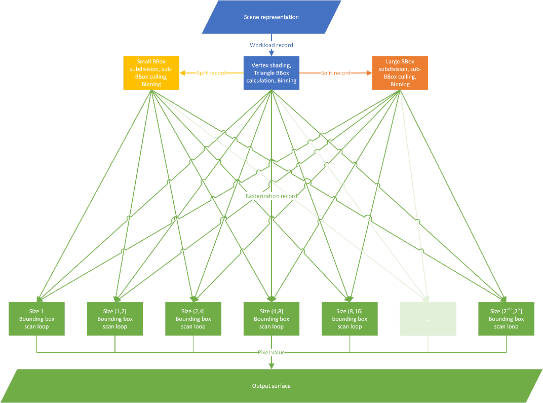
Below is the resulting explicit algorithm graph which we’ll subsequently implement:
The basic data structure we’re using to provide the scene data for the algorithm is as follows:
struct Workload{    uint offsetIndex;  // local cluster location in the global shared index buffer    uint offsetVertex; // local cluster location in the global shared vertex buffer                     // (indices are cluster local)    uint startIndex;   // start of the triangle-range in the index buffer    uint stopIndex;    // end of the triangle range in the index buffer, inclusive
    float4 vCenter;    float4 vRadius;
    matrix mWorldCurrent;    matrix mWorldPrevious;};
The Workload item describes a single object to be rasterized. The indices and vertices are all in one continuously accessible buffer, because it allows us to to get away with the traditional binding paradigm of DirectX, binding just two buffer descriptors. You can opt for a bindless paradigm as well, and use descriptor indices instead of global buffer indices.
Apart from that, we also pass the object’s position and extent, as well as its current world matrix. For static objects we’d only need to transmit this buffer once, as none of the information changes over time, but for this project the data is small enough to be transferred every frame and we don’t complicate things further with the need to disambiguate dynamic objects.
We conduct frustum culling on the CPU, and write the active scene elements as an array of Workload items, then we launch the work graph.
Looking at the graph above, we need to implement three different stages from an algorithm perspective:
For the subdivision we have two launch signatures (fixed vs. dynamic), but the algorithm in the body of the nodes is the same. Similar with rasterization, while we have k different bins, it just groups the data to be more coherent, and doesn’t require us to have specialized implementations.
This is the root node of the graph. Which is also the entry point of the program. It has the character of a regular Compute Dispatch in which we launch as many threads as there are triangles but share the object’s ID and parameters, hence we annotate it being of type Broadcasting.
[Shader("node")][NodeLaunch("Broadcasting")][NodeMaxDispatchGrid(65535, 1, 1)][NodeIsProgramEntry][NumThreads(TRANSF_NUM_THREADS, 1, 1)]void TriangleFetchAndTransform( uint WorkgroupIndex : SV_GroupID, uint SIMDLaneIndex : SV_GroupIndex,The node is fed by the CPU similar to a indirect argument buffer, we’ll get to that later in the C++ section.
This is the node which amplifies bounding boxes, we start a dispatch-grid as large as the calculated sub-division, but share the encompassing origin bounding box and the triangle’s parameters, it’s also of Broadcasting type.
[Shader("node")][NodeLaunch("broadcasting")]#if (EXPANSION == 1) // fixed expansion[NodeDispatchGrid(1, 1, 1)] // has the size of one wave, consumes nodispatch parameters[NumThreads(SPLITR_NUM_THREADS, 1, 1)]void SplitFixed(#elif (EXPANSION == 2) // dynamic expansion[NodeMaxDispatchGrid(240, 135, 1)] // can be very large, consumesdispatch parameters[NumThreads(SPLITR_NUM_THREADS, 1, 1)]void SplitDynamic(#else[NodeMaxDispatchGrid(240, 135, 1)][NumThreads(SPLITR_NUM_THREADS, 1, 1)]void Split(#endif uint WorkSIMDIndex : SV_DispatchThreadID, // use only one dimension to allow optimizations of the dispatchTo generate different signature (and function name) permutations we use preprocessor conditions and compile the node from the same code multiple times. Because we’re using different function signatures for fixed and dynamic nodes, they are not compatible/interchangeable with each other according to the current revision of the specification. Because of this we are unable to use a binning/indexing mechanism to target them, and have to explicitly relay data to one other the other.
The leaf node(s) of the graph are the rasterizers. Every thread works on it’s own bounding box and triangle, and there’s no useful information that could be shared between them. This node is of Thread type.
[Shader("node")][NodeLaunch("thread")][NodeID("Rasterize", TRIANGLE_BIN)] // indicate position in a node-array, passed in as a preprocessor symbol while compiling the nodevoid Rasterize(A Thread launch node is not controlled by an explicit argument about the size of the working set, instead the implementation operates a bit like a producer consumer queue. Once enough work has accumulated to launch a SIMD wave it will be launched with as many individual parameters as there are lanes. This is quite efficient, because the optimal number of launched treads can be chosen internally, and we don’t need to have perfect knowledge of the conditions. For example, this value can be distinct between architectures, or even SKUs. Or sometimes it’s better for the scheduler to kick out work to prevent stalls, recover allocations, or to prime a shader program on a SIMD unit.
Because the rasterizers are all identical in terms of code, we can use Workgraph’s powerful concept of node-arrays here: instead of redirecting work to nodes explicitly via conditional constructs (if/else, switch, …), this concept works similar to jump tables.
What’s left to do is defining the connections between the nodes. This is specified explicitly in a top down fashion: the outputs point explicitly to the nodes they target. To ensure these connections are valid, both inputs and outputs specify which data structure they are carrying, so that the runtime can verify that the connection is a valid one. The result is a directed acyclic graph.
The declarations of inputs and outputs are part of the function parameter declaration, including their local annotations. This can make Workgraph function signatures really big. In the following I will only show the particular part of the function signature related to the data record we’re explaining. In the code you’ll see them all together in one big block.
First we define how we feed data from the application into the graphs root node. Because the root node is of Broadcasting type, we use the required SV_DispatchGrid semantics in the data declaration. The workload-offset pointing to the global workload buffer is similar to a root signature constant (it’s the same over all invocations).
struct DrawRecord{    // index into the global scene buffer containing all Workload descriptors    uint  workloadOffset;
    uint3 DispatchGrid : SV_DispatchGrid;};
Now we declare this struct to be the type used for inputs into our root node function signature:
void TriangleFetchAndTransform( // Input record that contains the dispatch grid size. // Set up by the application. DispatchNodeInputRecord<DrawRecord> launchRecord,When we combine dispatch global parameters with dispatch local parameters, we can know exactly on which triangle every thread is suppose to work on.
Next we define how we pass data from our root node into the bounding box subdivision nodes. Because we use two different node types for this (a fixed Dispatch and a dynamic Dispatch, with incompatible function signatures), we also want to declare two different types of data structures. The dynamic Dispatch one has to use the required SV_DispatchGrid semantics in the data declaration. The fixed Dispatch could also use one, because the compiler will silently clear out unused semantic parameters, but we keep two versions for clarity and unambiguous compile time verification.
struct SplitDynamicRecord{    uint3 DispatchGrid : SV_DispatchGrid;
    // Triangle equation, bbox and interpolateable values    struct TriangleStateStorage tri;
    uint2 DispatchDims; // 2D grid range processed by this 1D dispatch    uint2 DispatchFrag; // 2D size of the subdividing bounding boxes};
struct SplitFixedRecord{ // Triangle equation, bbox and interpolateable values struct TriangleStateStorage tri;
uint2 DispatchDims; // 2D grid range processed by this 1D dispatch uint2 DispatchFrag; // 2D size of the subdividing bounding boxes};These two record types are then added to our root node’s function signature as individual outputs. For each output we have to annotate a couple of more things:
The former allows the allocator to switch allocation strategy depending on the situation, and the latter establishes unmistakably where the data goes.
void TriangleFetchAndTransform(    [MaxRecords(TRANSF_NUM_THREADS)] // N threads that each output 1 bbox-split    [NodeID("SplitFixed")]    NodeOutput<SplitFixedRecord> splitFixedOutput,
    [MaxRecords(TRANSF_NUM_THREADS)] // N threads that each output 1 bbox-split    [NodeID("SplitDynamic")]    NodeOutput<SplitDynamicRecord> splitDynamicOutput,
Then we declare this struct to be the type used for inputs into our subdivision node function signature:
void SplitFixed/Dynamic( // Input record that may contain the dispatch grid size. // Set up by TriangleFetchAndTransform. #if (EXPANSION == 1) // fixed expansion DispatchNodeInputRecord<SplitFixedRecord> splitRecord, #else // dynamic expansion DispatchNodeInputRecord<SplitDynamicRecord> splitRecord, #endifWe don’t change the body of the function, as it’s doing the same operations, and the parameters have been kept identical. instead we just specialize how it is called via the function signature.
Finally we define how we pass data from all of the nodes higher up in the graph into the rasterizer. The only data that’s left now, necessary for the rasterization loop, is really only the triangle equation, the bounding box to scan, and the values we like to interpolate.
struct RasterizeRecord{ // Triangle equation, bbox and interpolateable values struct TriangleStateStorage tri;};Although, as we planned in the beginning of the article, we want to collect data with similar performance characteristics together. The native Workgraph construct to achieve this is the output array. So far we’ve only targeted individual outputs. Output-arrays can be understood as bundles of outputs bound together. Instead of flow control we use an index to choose to which one to output to. When there are only a couple of outputs it might not make much of a difference, but once there are a couple of hundred of outputs involved, it becomes highly inefficient to branch. We specify the size of the output array in the annotations of the output together with output limits and output node name. Just like with multiple outputs, it’s not a requirement to select just a single option and feed data mutually exclusive. If an algorithm requires you to feed multiple outputs (or multiple slots in the output-array) with data, that’s perfectly fine. Just remember to adjust your peak output size.
void TriangleFetchAndTransform( [MaxRecords(TRANSF_NUM_THREADS)] // N threads that each output 1 triangle [NodeID("Rasterize")] [NodeArraySize(TRIANGLE_BINS)] // TRIANGLE_BINS defined by application // during compilation NodeOutputArray<RasterizeRecord> triangleOutputand:
void SplitFixed/Dynamic( [MaxRecords(SPLITR_NUM_THREADS)] // N threads that each output 1 triangle [NodeID("Rasterize")] [NodeArraySize(TRIANGLE_BINS)] // TRIANGLE_BINS defined by application // during compilation NodeOutputArray<RasterizeRecord> triangleOutputAlthough we may arrive at the rasterization node by different paths, the structure is the same, and the declaration very straightforward:
void Rasterize( ThreadNodeInputRecord<RasterizeRecord> triangleRecordJust like in a regular Compute algorithm, we’ll write out rasterized outputs to a UAV, and that doesn’t need a special declaration in Workgraphs.
With the inputs and outputs declared and ready to be used, we can implement the i/o. It’s fairly straightforward and I will not go through all instances.
If you have single input (as in the case for Broadcasting and Thread), we can call a simple getter on the declared input:
uint workloadOffset = launchRecord.Get().workloadOffset;That’s all there is to it. For Coalescing launches you’d just need to pass the index of the element you want to retrieve to the getter.
Outputting is slightly more complex. As dictated by the specification, you have to call the output record allocator in a coherent manner (all lanes leave, or none). To allow lane individual allocation, the API accepts a oolean to indicate if you really want to have a record, or if it’s a dummy allocation.
Let’s take a look at the outputting code of the root node:
const uint triangleBin                             = ts.triangleBBBin; // calculated bin, if not too largeconst bool allocateRasterRecordForThisThread       = ts.triangleValid; // true if not too largeconst bool allocateSplitDynamicRecordForThisThread = !allocateRasterRecordForThisThread & (DispatchGrid.x != 1); // too large, and many work groups necessary for subdivisionconst bool allocateSplitFixedRecordForThisThread   = !allocateRasterRecordForThisThread & (DispatchGrid.x == 1); // too large, but only one work group necessary for subdivision
// call allocators outside of branch scopes, the boolean indicates if we want a real record or notThreadNodeOutputRecords<RasterizeRecord> rasterRecord =    triangleOutput[triangleBin]      .GetThreadNodeOutputRecords(allocateRasterRecordForThisThread);ThreadNodeOutputRecords<SplitDynamicRecord> splitterDynamicRecord =    splitDynamicOutput      .GetThreadNodeOutputRecords(allocateSplitDynamicRecordForThisThread);ThreadNodeOutputRecords<SplitFixedRecord> splitterFixedRecord =    splitFixedOutput      .GetThreadNodeOutputRecords(allocateSplitFixedRecordForThisThread);
// fill the acquired output records, here we branch according to the conditionsif (allocateRasterRecordForThisThread){    rasterRecord.Get().tri = StoreTriangleState(ts);}else if (allocateSplitFixedRecordForThisThread){    splitterFixedRecord.Get().DispatchDims = DispatchDims;    splitterFixedRecord.Get().DispatchFrag = DispatchFrag;    splitterFixedRecord.Get().tri = StoreTriangleState(ts);}else if (allocateSplitDynamicRecordForThisThread){    splitterDynamicRecord.Get().DispatchGrid = DispatchGrid;    splitterDynamicRecord.Get().DispatchDims = DispatchDims;    splitterDynamicRecord.Get().DispatchFrag = DispatchFrag;    splitterDynamicRecord.Get().tri = StoreTriangleState(ts);}
// call completion outside of branch scopes, this allows the scheduler to start processing themrasterRecord.OutputComplete();splitterDynamicRecord.OutputComplete();splitterFixedRecord.OutputComplete();
We have three possible output scenarios:
Because we’re taking care not to branch around these calls, it looks a bit verbose, but there’s not much complexity to it. The record you’ll get from the output allocator is of the same type as the input records that you receive through the function. You need to call the getter in the same way. If you allocate multiple entries (not in this project), then you pass the index of the sub-allocation record that you want to access, same as with the record collection given to you in a Coalescing launch.
With this we have everything work graphs-specific implemented in our shader code. In the next chapter we’re going to take a look how to kick off the work graph from the CPU-side.
Creating a Workgraph program in D3D12 is a bit different than for a regular Graphics or Compute pipeline State Object. Schematically it’s similar to creating a State Object for raytracing (for which you also register a large amount of sub-programs).
First we’ll define the description of our Workgraph, and specify which is the entry point/root node:
D3D12_NODE_ID entryPointId = {    .Name = L"TriangleFetchAndTransform", // name of entry-point/root node    .ArrayIndex = 0,};
D3D12_WORK_GRAPH_DESC workGraphDesc = {    .ProgramName = L"WorkGraphRasterization",    .Flags = D3D12_WORK_GRAPH_FLAG_INCLUDE_ALL_AVAILABLE_NODES,    .NumEntrypoints = 1,    .pEntrypoints = &entryPointId,    .NumExplicitlyDefinedNodes = 0,    .pExplicitlyDefinedNodes = nullptr};
Then we compile all of our nodes into individual shader blobs, adjusting preprocessor symbols to receive exactly the permutation we want in-between:
CompileShaderFromFile(sourceWG, &defines,    "TriangleFetchAndTransform", "-T lib_6_8" OPT, &shaderComputeFrontend);
CompileShaderFromFile(sourceWG, &defines,    "SplitDynamic", "-T lib_6_8" OPT, &shaderComputeSplitter[0]);CompileShaderFromFile(sourceWG, &defines,    "SplitFixed", "-T lib_6_8" OPT, &shaderComputeSplitter[1]);
for (int triangleBin = 0; triangleBin < triangleBins; ++triangleBin)    CompileShaderFromFile(sourceWG, &defines,        "Rasterize", "-T lib_6_8" OPT, &shaderComputeRasterize[triangleBin);
The function names we specify here have to match the ones in the HLSL source code, so that the compiler knows which part of the source we want. You can see here that for the splitter we can use explicit function names, because we switch their names in the HLSL. For the rasterize function, we won’t do this, because it’s impractical for large numbers of nodes. Remember we have potentially hundreds of them!
Instead, we use a neat feature of the API: changing function names when linking the program, but more on that in a bit.
After we have compiled all of the individual shader blobs, we can register them as sub-objects for the work graphs program:
std::vector<D3D12_STATE_SUBOBJECT> subObjects = {    {.Type = D3D12_STATE_SUBOBJECT_TYPE_GLOBAL_ROOT_SIGNATURE,   .pDesc = &globalRootSignature},    {.Type = D3D12_STATE_SUBOBJECT_TYPE_WORK_GRAPH,   .pDesc = &workGraphDesc},};
D3D12_DXIL_LIBRARY_DESC shaderComputeFrontendDXIL = {    .DXILLibrary = shaderComputeFrontend,    .NumExports = 0,    .pExports = nullptr};
subObjects.emplace_back(D3D12_STATE_SUBOBJECT_TYPE_DXIL_LIBRARY, &shaderComputeFrontendDXIL); // move into persistent allocation
D3D12_DXIL_LIBRARY_DESC shaderComputeSplitter0DXIL = {    .DXILLibrary = shaderComputeSplitter[0],    .NumExports = 0,    .pExports = nullptr};
subObjects.emplace_back(D3D12_STATE_SUBOBJECT_TYPE_DXIL_LIBRARY, &shaderComputeSplitter0DXIL); // move into persistent allocation
D3D12_DXIL_LIBRARY_DESC shaderComputeSplitter1DXIL = {    .DXILLibrary = shaderComputeSplitter[1],    .NumExports = 0,    .pExports = nullptr};
subObjects.emplace_back(D3D12_STATE_SUBOBJECT_TYPE_DXIL_LIBRARY, &shaderComputeSplitter1DXIL); // move into persistent allocation
So far so good. Now we want to register the rasterizer shader blobs, and those we have to rename. The linker will automatically match function names with the output array declaration that we gave in HLSL:
[NodeID("Rasterize")]NodeOutputArray<RasterizeRecord> triangleOutputThe pattern which the matcher follows is “<function name>_<index>”. We will specify that we want the “Rasterize” to be renamed to “Rasterize_0” and so on in the following:
for (int triangleBin = 0; triangleBin < triangleBins; ++triangleBin){    auto entryPoint = L"Rasterize";
    // Change "Rasterize" into "Rasterize_k"    refNames.emplace_back(std::format(L"{}_{}", entryPoint, triangleBin)); // move into persistent allocation
    // Tell the linker to change the export name when linking    D3D12_EXPORT_DESC shaderComputeRasterizeExport = {        .Name = refNames.back().c_str(),        .ExportToRename = entryPoint,        .Flags = D3D12_EXPORT_FLAG_NONE    };
    expNames.emplace_back(shaderComputeRasterizeExport); // move into persistent allocation
    D3D12_DXIL_LIBRARY_DESC shaderComputeRasterizeDXIL = {        .DXILLibrary = shaderComputeRasterize[triangleBin],        .NumExports = 1,        .pExports = &expNames.back()    };
    libNames.emplace_back(shaderComputeRasterizeDXIL); // move into persistent allocation
    subObjects.emplace_back(D3D12_STATE_SUBOBJECT_TYPE_DXIL_LIBRARY, &libNames.back());}
Additionally there’s a bit of code to prevent dangling points from out-of-scope deallocations.
Now we have collected and defined all necessary information to create our Workgraphs program:
const D3D12_STATE_OBJECT_DESC stateObjectDesc = {    .Type = D3D12_STATE_OBJECT_TYPE_EXECUTABLE,    .NumSubobjects = static_cast<UINT>(subObjects.size()),    .pSubobjects = subObjects.data()};
ThrowIfFailed(m_pDevice->CreateStateObject(&stateObjectDesc, IID_PPV_ARGS(&m_pipelineWorkGraph)));
It’s certainly more complicated to set up than one of the predefined hardware pipeline stages (VS, PS, CS etc.), but it allows you to flexibly assemble a variety of different Workgraphs from common building blocks without the need to leak the specification of that variety into your HLSL code.
As we said in the beginning, one of the beneficial capabilities of Workgraphs, is that it allows you to make allocations to pass data from one node to the next. But the memory pool from which the implementation draws it’s allocations from, is not some hidden implicit one. After we got the Workgraph State Object we have to find out how large that memory pool should be in total, and we also have to allocate and provide a buffer to the implementation ourselves:
ComPtr<ID3D12WorkGraphProperties> workGraphProperties;ThrowIfFailed(m_pipelineWorkGraph->QueryInterface(IID_PPV_ARGS(&workGraphProperties)));
D3D12_WORK_GRAPH_MEMORY_REQUIREMENTS workGraphMemoryRequirements;workGraphProperties->GetWorkGraphMemoryRequirements(0, &workGraphMemoryRequirements);
const auto workGraphBackingMemoryResourceDesc = CD3DX12_RESOURCE_DESC::Buffer(workGraphMemoryRequirements.MaxSizeInBytes);
const auto defaultHeapProps = CD3DX12_HEAP_PROPERTIES(D3D12_HEAP_TYPE_DEFAULT);
ThrowIfFailed(m_pDevice->CreateCommittedResource(    &defaultHeapProps,    D3D12_HEAP_FLAG_NONE,    &workGraphBackingMemoryResourceDesc,    D3D12_RESOURCE_STATE_COMMON,    nullptr,    IID_PPV_ARGS(&m_memoryWorkGraph)));
const D3D12_GPU_VIRTUAL_ADDRESS_RANGE backingMemoryAddrRange = {    .StartAddress = m_memoryWorkGraph->GetGPUVirtualAddress(),    .SizeInBytes = workGraphMemoryRequirements.MaxSizeInBytes,};
The size of the backing memory depends on the structure of your Workgraph: how many outputs are there? what’re the types of the outputs? etc. The memory size will be sufficient for the Workgraph implementation to always have the ability to make forward progress.
Finally we are ready to start the Workgraph on the GPU. We have:
Again, setting the Workgraphs implementation is requiring us to set up a couple of structures to tell the runtime exactly what we want to happen:
ComPtr<ID3D12WorkGraphProperties> workGraphProperties;ThrowIfFailed(m_pipelineWorkGraph->QueryInterface(IID_PPV_ARGS(&workGraphProperties)));
ComPtr<ID3D12StateObjectProperties1> workGraphProperties1;ThrowIfFailed(m_pipelineWorkGraph->QueryInterface(IID_PPV_ARGS(&workGraphProperties1)));
D3D12_WORK_GRAPH_MEMORY_REQUIREMENTS workGraphMemoryRequirements;workGraphProperties->GetWorkGraphMemoryRequirements(0, &workGraphMemoryRequirements);
// Define the address and size of the backing memoryconst D3D12_GPU_VIRTUAL_ADDRESS_RANGE backingMemoryAddrRange = {    .StartAddress = m_memoryWorkGraph->GetGPUVirtualAddress(),    .SizeInBytes = workGraphMemoryRequirements.MaxSizeInBytes,};
// Backing memory only needs to be initialized onceconst D3D12_SET_WORK_GRAPH_FLAGS setWorkGraphFlags =m_memoryInitialized ? D3D12_SET_WORK_GRAPH_FLAG_NONE                    : D3D12_SET_WORK_GRAPH_FLAG_INITIALIZE;m_memoryInitialized = true;
const D3D12_SET_WORK_GRAPH_DESC workGraphProgramDesc = {    .ProgramIdentifier = workGraphProperties1->GetProgramIdentifier(L"WorkGraphRasterization"),    .Flags = setWorkGraphFlags,    .BackingMemory = backingMemoryAddrRange};
const D3D12_SET_PROGRAM_DESC programDesc = {    .Type = D3D12_PROGRAM_TYPE_WORK_GRAPH,    .WorkGraph = workGraphProgramDesc};
// Set the program and backing memorypCommandList->SetProgram(&programDesc);
// Submit all of our DrawRecords in one batch-submissionconst D3D12_NODE_CPU_INPUT nodeCPUInput {    .EntrypointIndex = 0,    .NumRecords = UINT(m_Arguments.size()),    .pRecords = (void*)m_Arguments.data(),    .RecordStrideInBytes = sizeof(DrawRecord),};
const D3D12_DISPATCH_GRAPH_DESC dispatchGraphDesc = {    .Mode = D3D12_DISPATCH_MODE_NODE_CPU_INPUT,    .NodeCPUInput = nodeCPUInput,};
pCommandList->DispatchGraph(&dispatchGraphDesc);
This now launches as many Workgraph instances, as we have objects in the scene. Every Workgraph instance goes through as many vertices as there are in each object in it’s root-node, and continues through the graph until it arrives at the leafs, where we write out our rasterized and interpolated values to a screen-sized UAV.
As we’ve reached the end of the article, let’s take a look at the results, and if everything works out as we anticipated. In the implementation in the rasterizer repository we are providing you with a variety of controls, so that you can explore the performance differences in real-time.
This scene if from the glTFSample repository. It’s Crytek’s Sponza scene. It has some very large triangles, and many smaller ones. Darker shades indicate smaller bounding boxes.
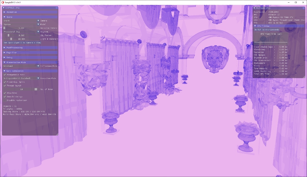
Times are given in 10ns ticks. The tested GPU is a 7900 XTX. The tested Driver is 23.20.11.01. For better visibility, there’s a graph plotted with the log10(ratio) against a monolithic (plain GPU SIMD) implementation.
| 10ns ticks | log10(ratio) |
|---|---|
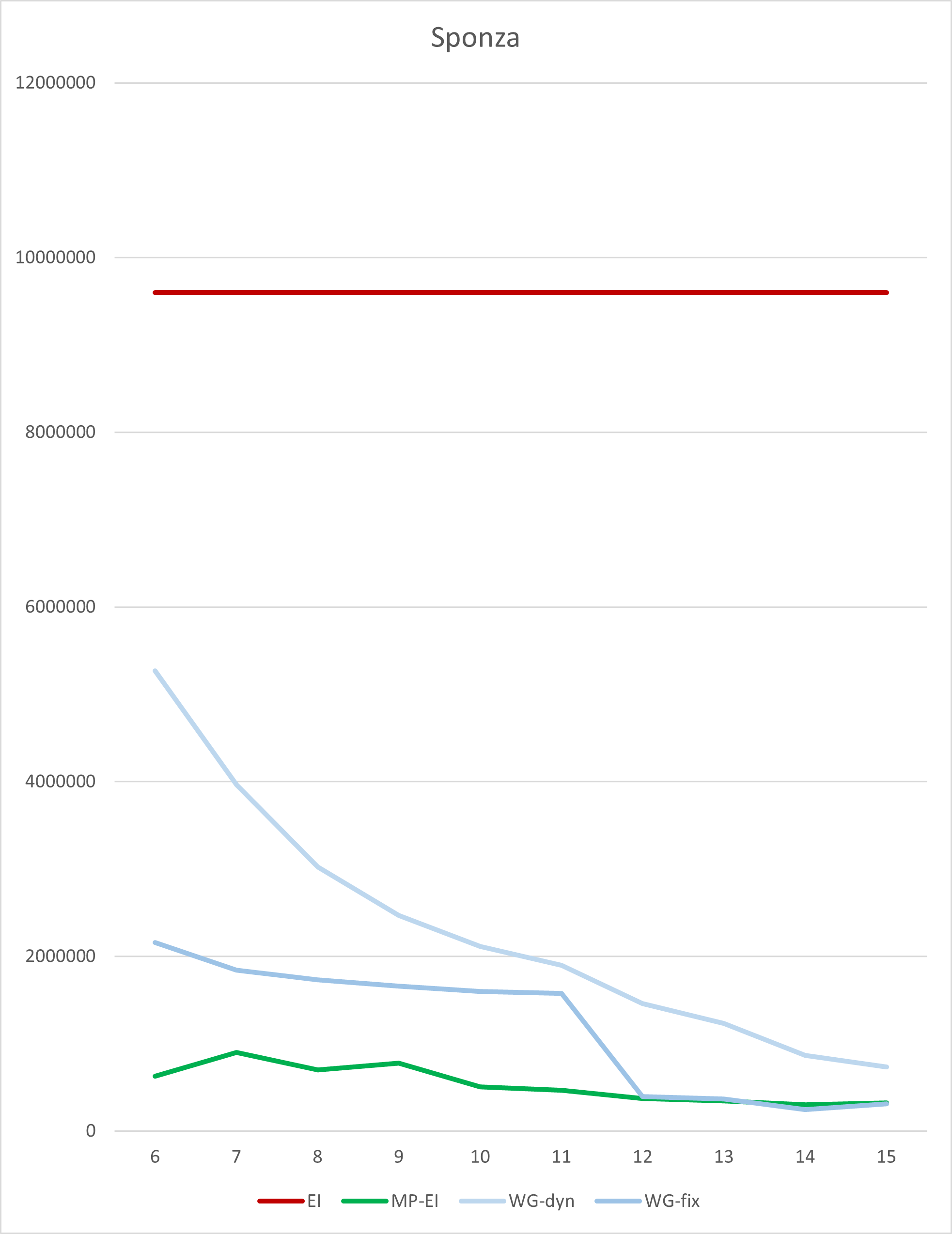 |  |
| bins | monolithic ExIn | multi-pass ExIn | dynamic WoGr | fixed WoGr |
|---|---|---|---|---|
| 6 | 9598764 | 625700 | 5267600 | 2158076 |
| 7 | 9598764 | 898932 | 3964992 | 1842596 |
| 8 | 9598764 | 698976 | 3020956 | 1730860 |
| 9 | 9598764 | 776720 | 2466808 | 1661224 |
| 10 | 9598764 | 507876 | 2111640 | 1598632 |
| 11 | 9598764 | 467532 | 1896800 | 1575920 |
| 12 | 9598764 | 373704 | 1461440 | 395980 |
| 13 | 9598764 | 347604 | 1229584 | 368704 |
| 14 | 9598764 | 301444 | 863680 | 248180 |
| 15 | 9598764 | 320772 | 731676 | 310732 |
As you can see, performance differs significantly depending on the number of bins (and thus the maximum size of rasterized bounding boxes). But a sweet spot appears to be around 14 bins (which is about 214 = 16k pixels, 128x128 among it). The Workgraph implementation has a moderate sized backing buffer of ~130MB. It is more than ~38x faster than the monolithic ExecuteIndirect implementation. The fixed Dispatch variation outperforms the dynamic Dispatch only variation by ~3x.
If we’d compare against a complicated multi-pass ExecuteIndirect implementation, which is much less flexible in terms of memory consumption and eats a large amount of memory bandwidth, we still come out on top by ~1.2x.
The sample code for this tutorial is available on GitHub: https://github.com/GPUOpen-LibrariesAndSDKs/WorkGraphComputeRasterizer
To allow you to experiment with a large variety of scenes, it’s based on the glTFSample already available on GitHub: https://github.com/GPUOpen-LibrariesAndSDKs/glTFSample
A fantastic repository for glTF scenes for you to check out is also on GitHub: https://github.com/KhronosGroup/glTF-Sample-Models
The source codes touch on in this tutorial can be found here:
Links to third-party sites are provided for convenience and unless explicitly stated, AMD is not responsible for the contents of such linked sites, and no endorsement is implied. GD-98
Microsoft is a registered trademark of Microsoft Corporation in the US and/or other countries. Other product names used in this publication are for identification purposes only and may be trademarks of their respective owners.
DirectX is a registered trademark of Microsoft Corporation in the US and/or other countries.