AMD FidelityFX™ Variable Shading
AMD FidelityFX Variable Shading drives Variable Rate Shading into your game.
So far, we’ve covered how you can add mesh nodes to an existing work graphs application, and how the HelloMeshNodes sample uses them to draw the Koch snowflake fractal. Further, we’ve discussed some best practices and other tricks to get the most out of mesh nodes. In this section, we’re going to take a look at how the procedural mesh node sample uses work graphs and mesh nodes to generate and render a fully procedural world.
The procedural generation mesh node sample shows fully GPU-driven rendering at work. The entire world is fully procedurally generated every frame and rendered entirely on the GPU through multiple different mesh nodes. Many of the procedural effects, e.g., the procedural grass, bees and butterflies, are based on the GDC 2024 mesh nodes demo. You can find the full source code for the sample along with pre-built binaries here and you can learn more about the procedural effects of the GDC 2024 demo in our upcoming paper, which has been published at HPG 2024.
We also have a Work Graphs Ivy Generation sample available.
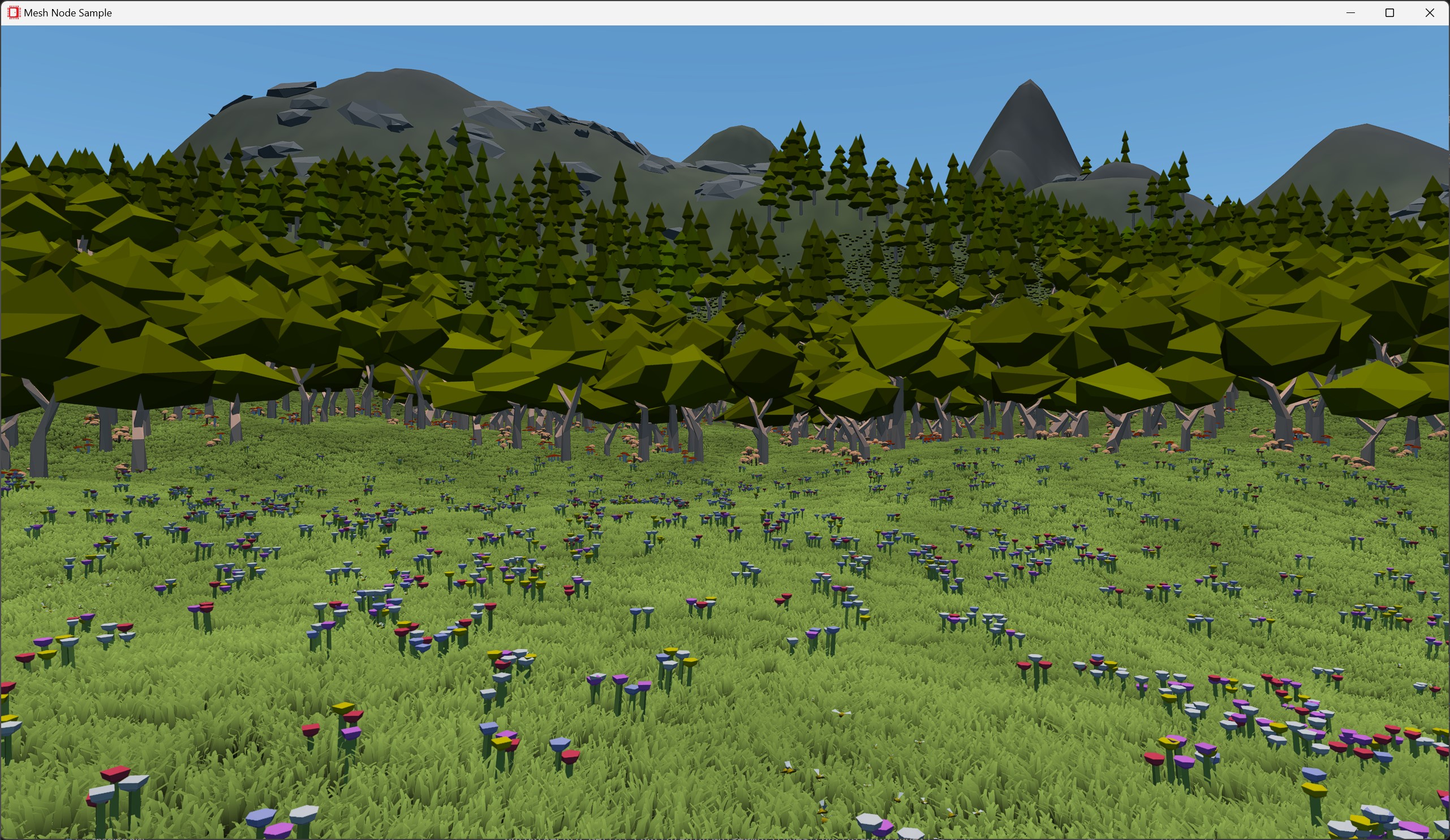
Generating an entire world procedurally on the GPU without work graphs is difficult, as limits for the overall output are often not known upfront. Work graphs in combination with mesh nodes greatly simplifies this. Dynamically scheduling work - including draws - on the fly, removes the need to reserve output memory for the entire world.
To generate a detailed world with coarse structures, like the terrain and fine details, like the grass, flowers and bees, we organize the world in a hierarchical grid. Each of these levels is represented with one node(-array) per level, with each level generating multiple records of the next lower level. Starting from the coarsest level, we have the following nodes:

World: entry node to the graph. This node projects the corners of the camera view frustum onto the -plane and computes the outer bounding box. This bounding box is quantized to the chunk grid spacing and is then used to launch a 2D grid of chunk thread groups. A visualization for this can be seen on the right.Chunk: handles a large square block of the world. Each chunk consists of one thread group with threads.
The entire thread group is responsible for invoking the terrain mesh node with the correct level of detail.
Each thread in a chunk is responsible for launching a tile.Tile[3]: node array of three different nodes, one for each biome type. Each tile consists of one thread group with threads. Each thread handles coarse-grained procedural generation, e.g. trees, flowers, rocks.DetailedTile: handles generation of a block of dense grass patches. You can find more information on how these grass patches are rendered in our procedural grass rendering blog post.
Organizing the procedural world generation into these multiple levels has several advantages. First and foremost, it allows us to cull non-visible grid-cells at every level and thereby reduce the overall workload. Secondly, we can split different procedural effects into different levels. Instead of having one large shader to generate the entire world, we can have specialized shaders (or nodes) to only generate certain aspects, such as the terrain, grass or trees. Work graphs in combination with mesh nodes allows us to combine and re-use these nodes in different ways, without needing to track memory allocations for them.
As mentioned above, tiles are classified into three different biomes: mountain, woodland and grassland.
Each of these biomes is represented by a different node in the Tile node array and has different characteristics for generating further procedural effects.
For example, the mountain biome generates clusters of trees and rocks, while the grassland biome generates flowers, bees, and butterflies.
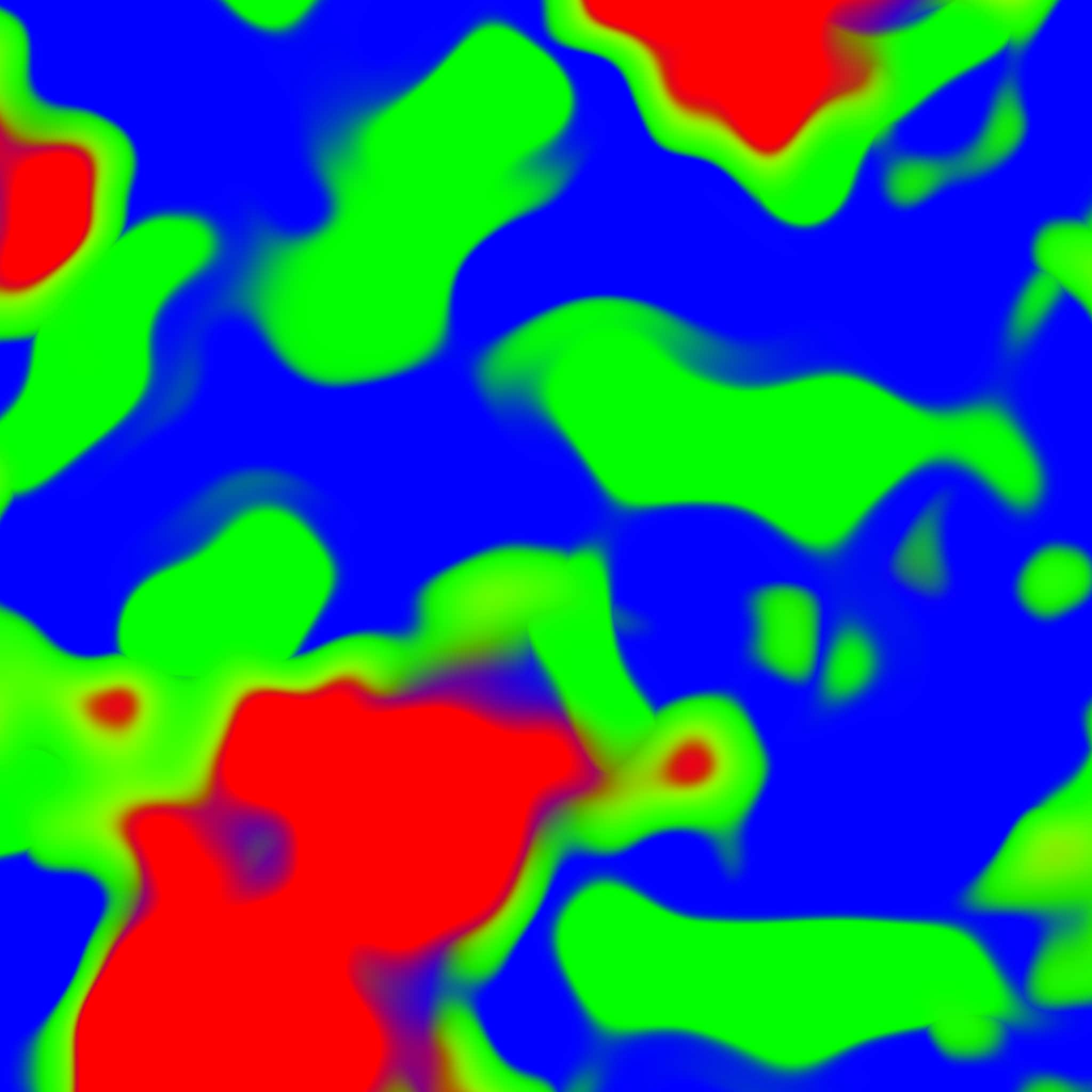
To classify each tile to a biome, we need a weight map for each biome.
We can procedurally generate such a map by layering perlin noise with different frequencies and amplitudes.
When combining the weight maps for different biomes, we can modify them, such that there will always be a dominant biome.
The result can be seen in the image on the right, with red representing the mountain biome, green representing the woodland biomes and blue the grassland biome.
You can find the source code for generating this map here.
Note that we do not store this map in a texture, but evaluate the GetBiomeWeights function anytime we need to sample the biome weight map.
We can then query this biome map at the center of each tile to determine its biome.
The resulting biome index is then used as an index into the Tile node array.
With node arrays, every thread in a Chunk thread group can output to a different node in this node array.
The resulting classification can be seen below.

As mentioned before, these biome specific tiles have different procedural generation characteristics:
MountainTile: The mountain tiles can generate rocks in flat areas and along mountain ridges. Additionally it can generate small clusters of pine trees if the terrain is not too steep.WoodlandTile: The woodland tile primarily generates trees. The type of tree (oak or pine) is determined by the steepness of the terrain and the distance to the next mountain biome.
A small cluster of mushrooms is also generated next to each tree.
Additionally, the woodland tile also generates sparse grass patches, which are replaced with detailed tiles if the camera is close enough.GrasslandTile: The grassland tile generates a meadow with flowers, bees and butterflies.
It uses the same logic as the woodland tile to generate sparse grass patches or detailed tiles.
Each thread can generate multiple flowers within the tile and a procedural swarm of bees is generated over some of the flowers.
Additionally, each thread can also generate a swarm of butterflies.We’ve seen how work graphs allows us to have a hierarchical structure for our generation logic and how we can split different generation steps, such as the biomes into dedicated nodes. Next, we’ll focus on some of the mesh nodes in the graph to see how we can actually draw our procedural world.
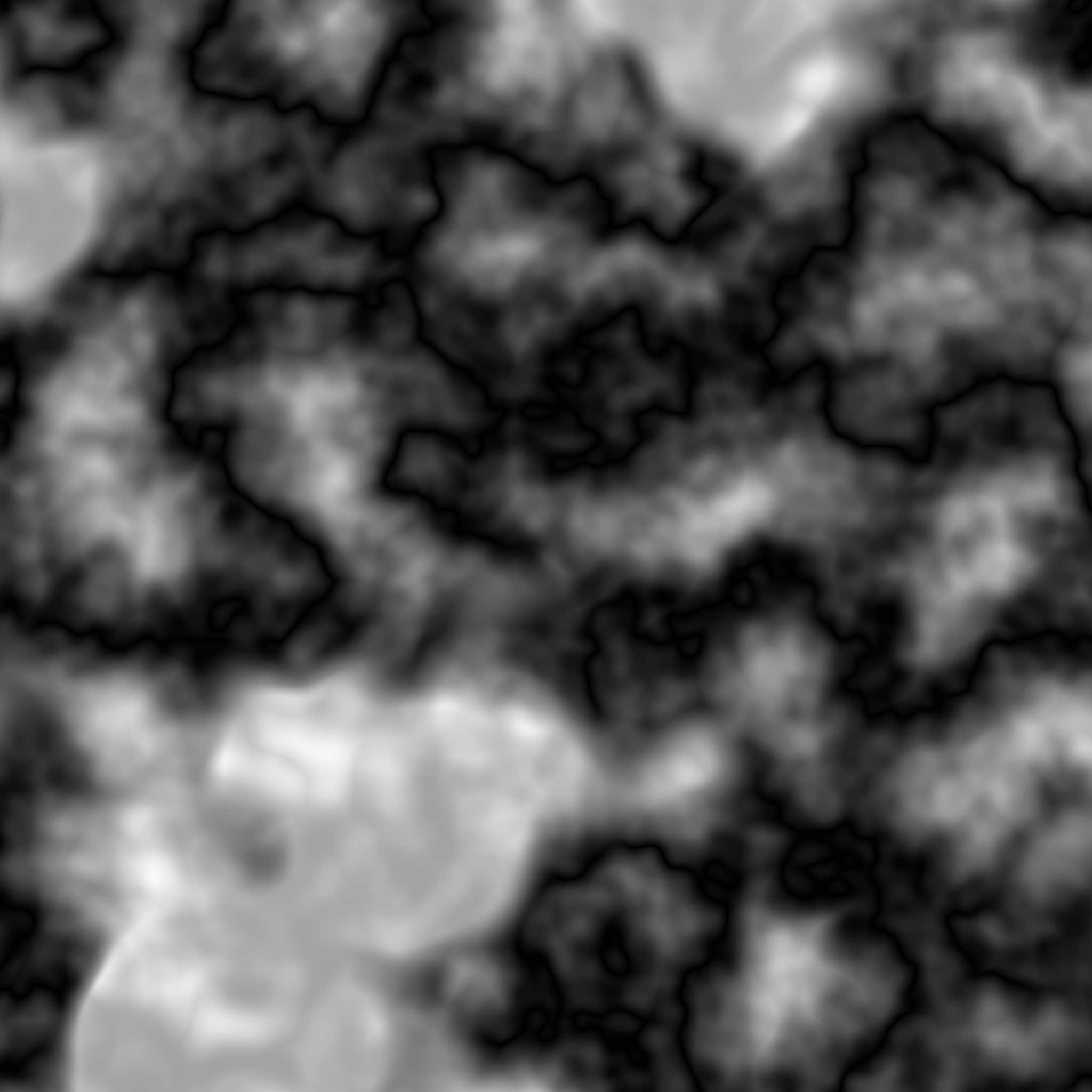
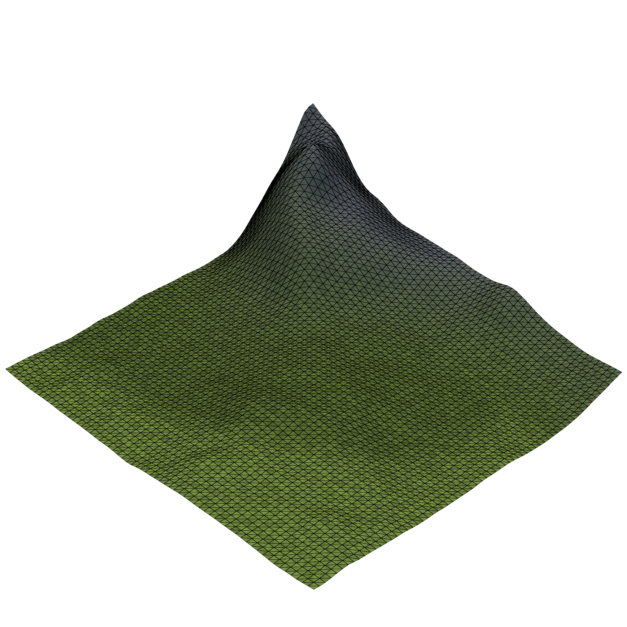
To generate and render a procedural terrain, we first need a heightmap, with which we can determine the height, and thus position of the terrain anywhere on the -plane. To generate such a heightmap, we again layer different frequencies of perlin noise, similar to the biome weight map that we generated earlier. Additionally, we can use the biome weight map to influence the terrain heightmap generation and raise the overall height level in the mountain biome. You can see the resulting heightmap on the right. Similar to the biome weight map, we do not store this map in memory, but evaluate its generation function anytime we need to sample the terrain height.
Rendering such a procedural heightmap terrain would often be implemented with tessellation shaders. As these are not supported in work graphs, we use a mesh shader instead. Each mesh shader thread group generates a grid section. Each of these grid sections consists of vertices, which are connected with triangles. We can then use multiple of these mesh shader thread groups to render a continuous, seamless terrain.
Launching the terrain mesh node is handled by the Chunk node.
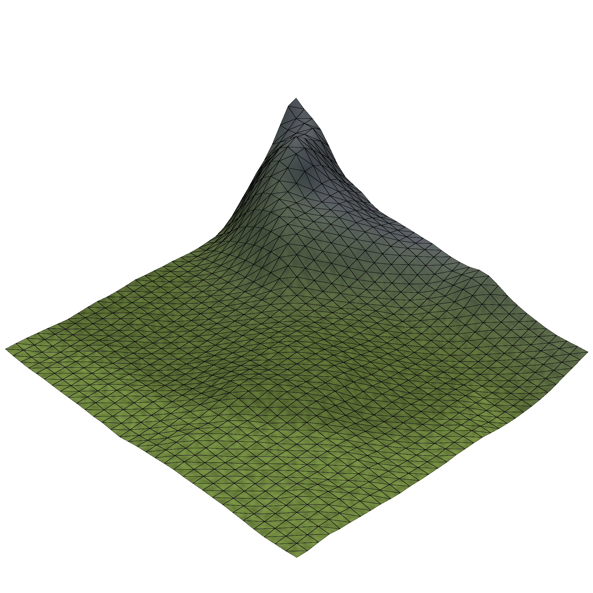
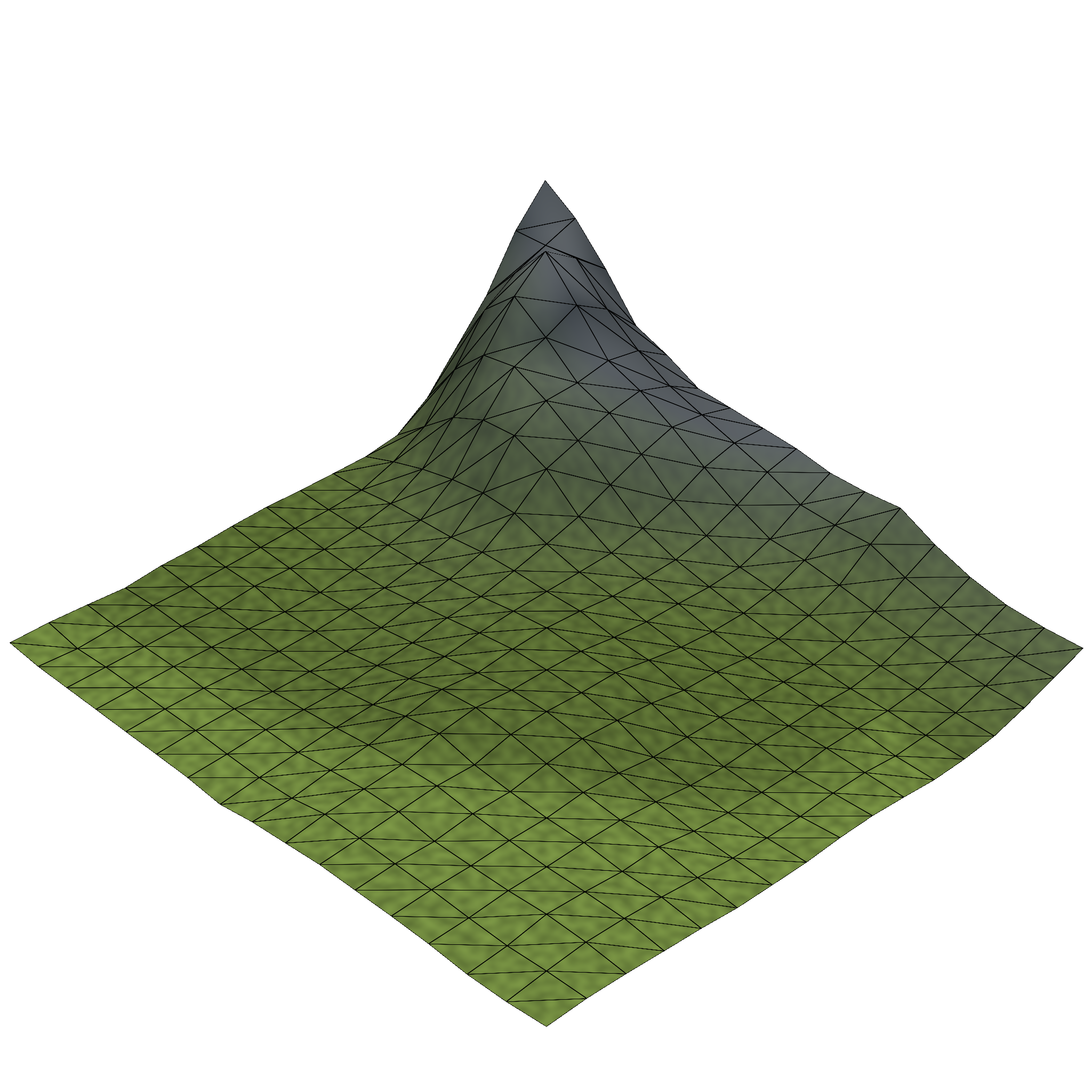
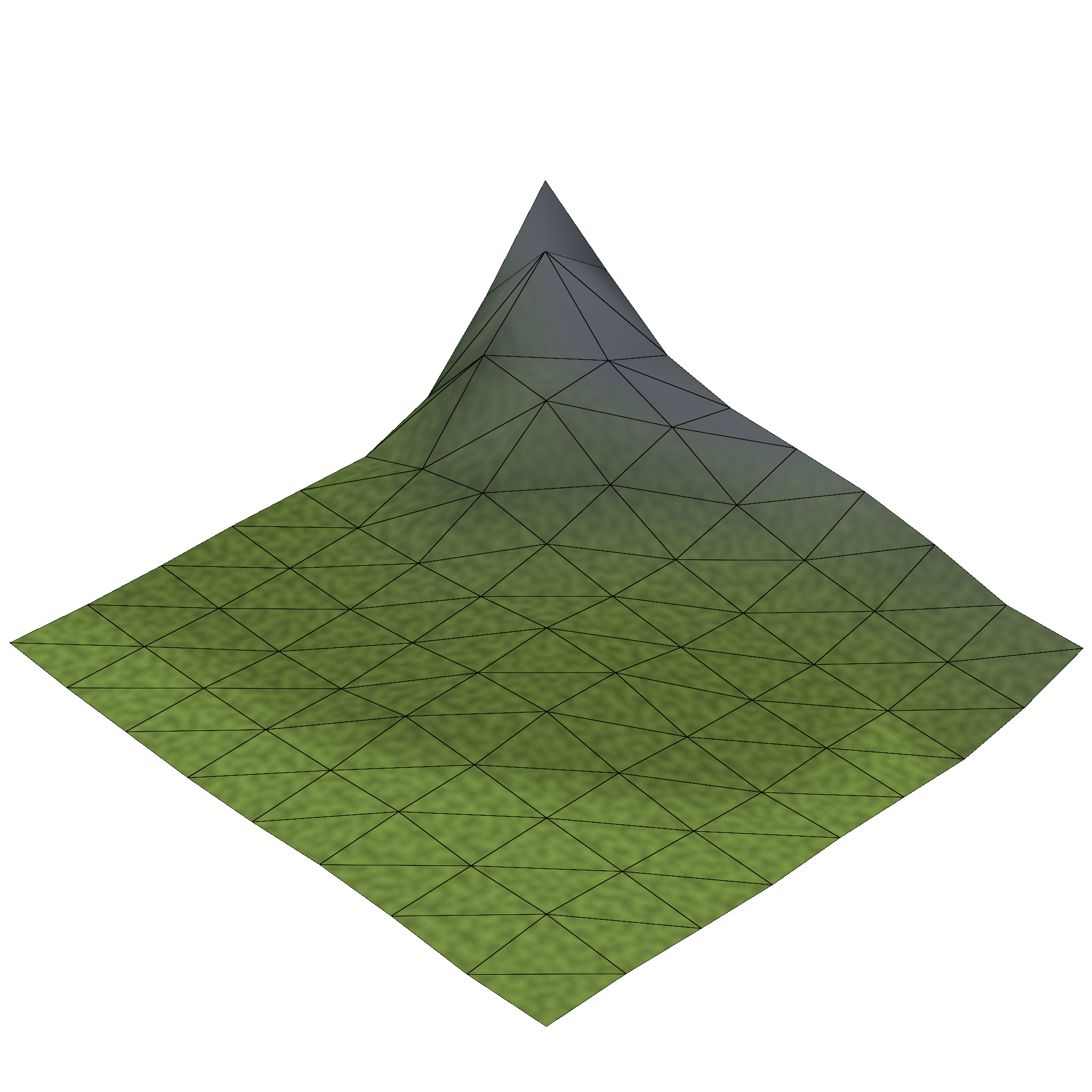
To achieve multiple levels of detail, each chunk can adjust the spacing between the terrain vertices and thereby the number of thread groups that are required to render the terrain in a chunk.
This ranges from mesh node thread groups per chunk for the highest level of detail, to just a single thread group for distant chunks.
| LOD 0 | LOD 1 | LOD 2 | LOD 3 |
|---|---|---|---|
 |  |  |  |
As outlined in the beginning, work graphs allow us to split the procedural generation into multiple, separate nodes. Such separation of concerns also allows us to build reusable components, i.e., nodes, to be used in different procedural effects. In the following, we’re going to look at how we can create a mesh node to render parametric splines of tree trunks and branches, and how such a node can serve as a building block to also render tree tops and rocks.
A tree trunk can be represented with a spline. Each spline is defined by a series of control points, which together form a curve in 3D space. To render a spline, we generate a ring of vertices at each control point and connect adjacent rings with triangles. Our spline thus has the following parameters:
With such a node in place, we can easily generate trees with different shapes and branches by modifying parameters of the spline or combining multiple splines together.
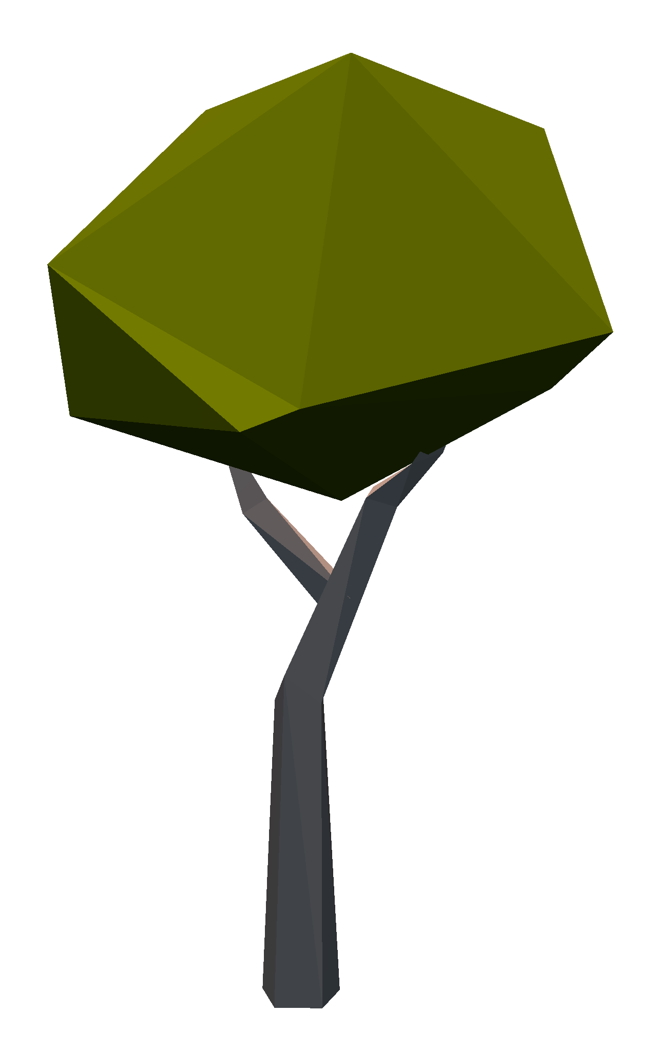
We can extend the spline mesh shader with a color and wind strength parameter for each spline. By adjusting the spline parameters to form a sphere and shading it green, we can also render the tree top for oak trees with the same mesh shader. For pine trees, we can arrange the control points in pairs and adjust the vertex ring radii to form a sawtooth-like shape. Rocks are - at least in the context of rendering them - just gray versions of the oak tree tops.
As described above, the procedural generation of the terrain mesh allows us to have different levels of detail. We can apply a similar concept to both the grass and flower generation in order to reduce the number of rendered triangles for distant objects.
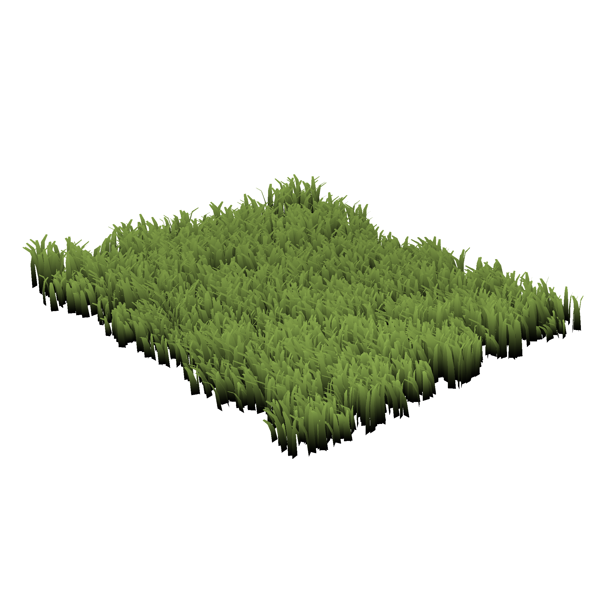
Grass
For the dense grass patches, we’re reusing the mesh shader from the procedural grass rendering blog post.
These dense grass patches are generated by the DetailedTile node.
Each detailed tile can generate up to grass patches, which up to two dense grass mesh shader thread groups per patch.
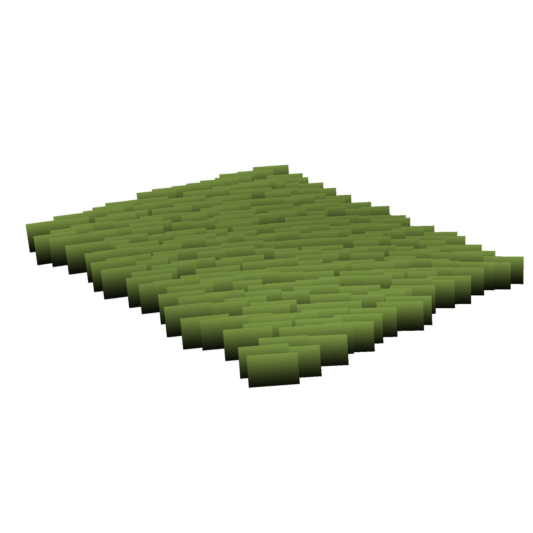
To reduce the number of thread groups and triangles required to render grass in a detailed tile, we introduce the following level of detail system:
Each detailed tile is replaced by a single sparse grass patch.
Each grass patch in the detailed tile is now rendered with a single quad (two triangles).
The sparse grass mesh shader can render a grid of these quads.
Thus, we now only need eight thread groups to render all the grass patches in the detailed tile.
The sparse grass is generated at the Tile level, to combine multiple sparse grass patches into a single record. See tips, tricks & best practices for more details.
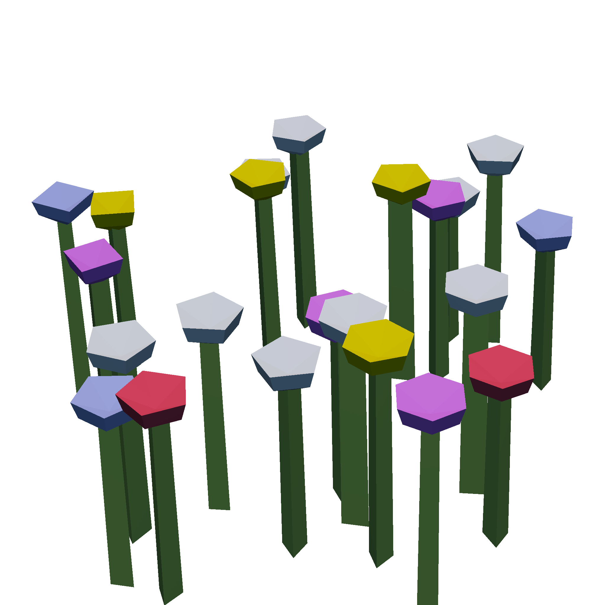
Flowers
Each flower patch can contain up to six flowers.
Thus, with a similar level of detail scheme of two triangles per flower, we can fit up to five flower patches in a single sparse flower mesh shader thread group.
Similar to the sparse grass, flowers are generated by the GrasslandTile node and multiple flower patches are combined into a single record.
DrawDenseGrassPatch | DrawSparseGrassPatch | DrawFlowerPatch[0] | DrawFlowerPatch[1] | |
|---|---|---|---|---|
 |  |  |  | |
| Thread Groups | ||||
| Vertices | ||||
| Triangles |

The World node is the entry node for our procedural world generation and uses the camera view frustum to launch a two-dimensional grid of Chunk thread groups.
To improve performance, this chunk grid is limited to only extend a certain distance away from the camera and is limited to a maximum of chunks.
As this grid follows the camera, we can see chunks appearing and disappearing at the far end of the camera view frustum.
To hide chunks popping in and out of view, we could increase the maximum chunk grid size or use effects like distance fog to hide the boundary of our chunk grid. For this sample, we instead decided to hide the end of the (generated) world by turning the world into a sphere. That said, our biome and heightmap generation allow for a virtually endless world, thus circumnavigating this sphere is not possible. In other words, we’re only creating an illusion of a spherical world.
To create this illusion, we transform every vertex position onto our imaginary sphere before projecting the vertex into clip space.
Performing this transform at such a late stage means we do not have to adjust any of our generation logic to this spherical space.
To transform a vertex position, we take its distance to the camera in the -plane () and its height above the -plane ().
We can find a position on our sphere with radius , such that the arc-length distance from the camera position is .
We offset this position along the sphere’s normal, scaled by .
For very distant vertices, we additionally scale towards zero, to ensure that even the tallest mountains disappear behind the horizon.
The resulting effect can be seen below.
And that’s it - we hope that this helps and encourages you to go out and try Mesh Nodes in Work Graphs. As always, we’d love to hear your feedback - this is a preview after all and things can still be changed before final release.
Links to third-party sites are provided for convenience and unless explicitly stated, AMD is not responsible for the contents of such linked sites, and no endorsement is implied. GD-98
Microsoft is a registered trademark of Microsoft Corporation in the US and/or other countries. Other product names used in this publication are for identification purposes only and may be trademarks of their respective owners.
DirectX is a registered trademark of Microsoft Corporation in the US and/or other countries.