Meet AMD FSR™ Technologies
Integrate our "Redstone" neural rendering technologies to take your game to new levels of fidelity and performance.
Integrate our "Redstone" neural rendering technologies to take your game to new levels of fidelity and performance.
Integrate our "Redstone" neural rendering technologies to take your game to new levels of fidelity and performance.
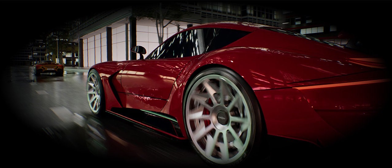
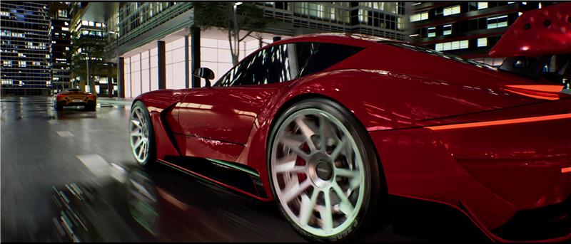
The AMD FSR™ "Redstone" SDK 2.2 update delivers ML-powered FSR Upscaling 4.1 and FSR Ray Regeneration 1.1 optimized for AMD RDNA™ 4 graphics, enabling higher visual fidelity and…
The AMD FSR Redstone SDK enables developers to integrate neural rendering technologies, including ML-powered upscaling, frame generation, denoising, and radiance caching, for…
Download the AMD FSR plugin for Unreal Engine, and learn how to install and use it.
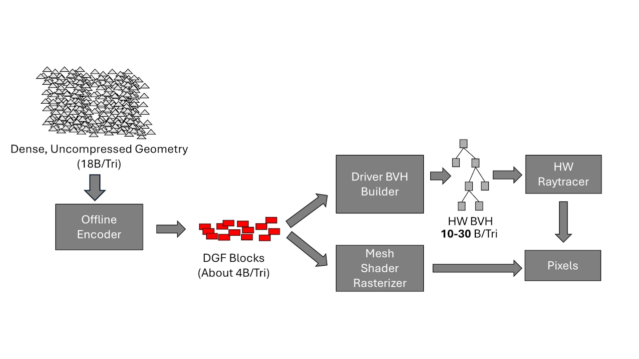
AMD is partnering with Samsung on a multivendor Vulkan extension for Dense Geometry Format (DGF) to help enable dramatically smaller geometry, reduced memory/latency for…
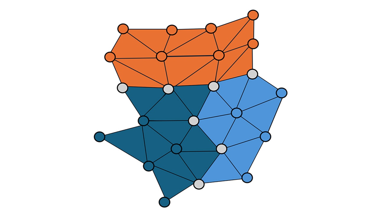
AMD DGF SuperCompression (DGFS) cuts DGF geometry file sizes while preserving exact block reconstruction and enabling fast decode to either DGF blocks or conventional meshlets for…
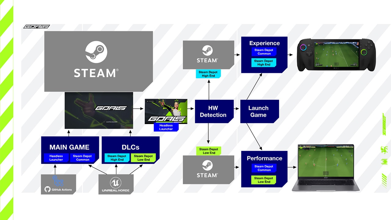
The first part of a developer-first look at how GOALS leverages AMD Ryzen APUs and the ADLX SDK to implement a system that reduces power, fan noise and carbon footprint across…
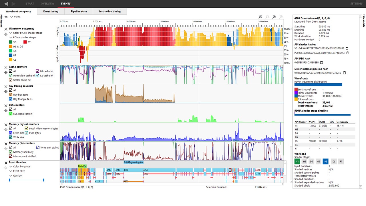
The latest version of the RDTS is designed to empower developers with enhanced capabilities for profiling, analyzing, and optimizing their GPU applications.
Youthcat Games overhauled the Dyson Sphere Program game's multithreading system, boosting performance by up to 88% through custom core binding, dynamic task allocation, and…
It is often difficult to know where to start when taking your first in the world of graphics. This guide is here to help with a discussion of first steps and a list of useful…
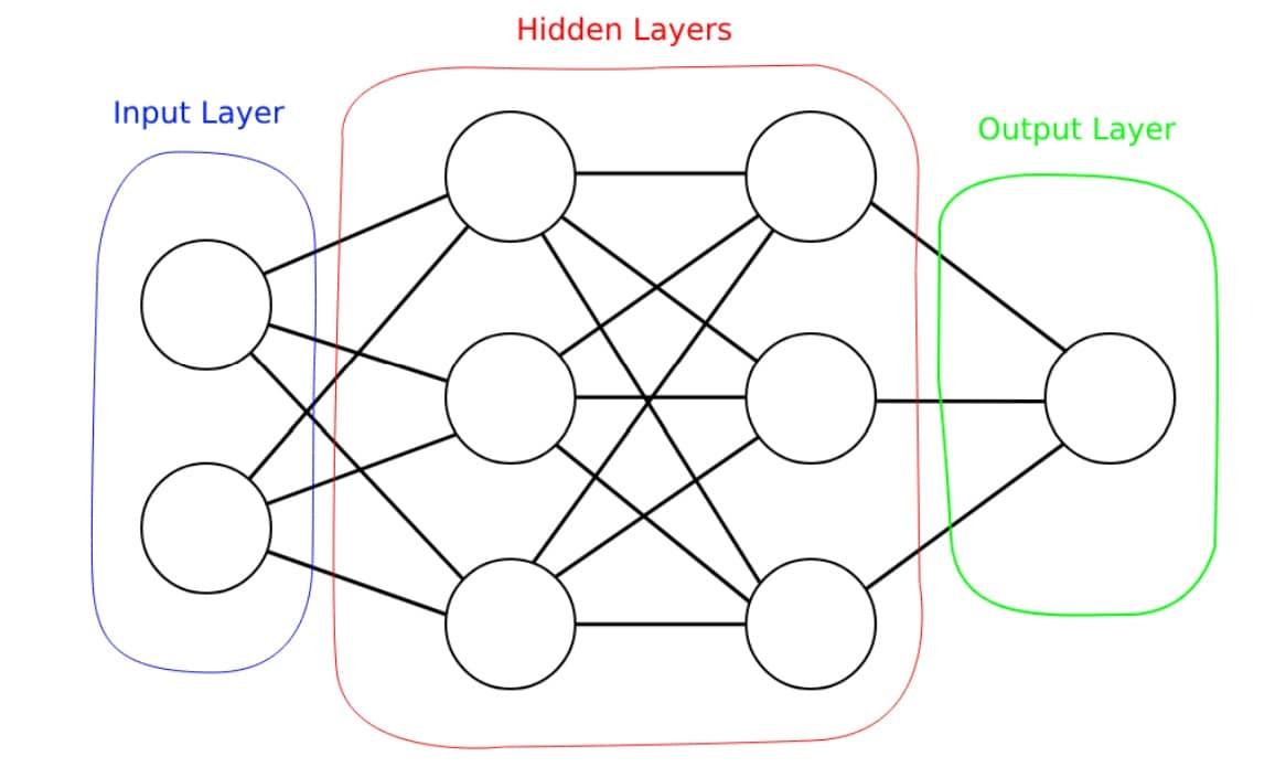
If you're a graphics dev looking to understand more about deep learning, this blog introduces the basic principles in a graphics dev context.
 | Introducing MiniDXNN: MLP library for DirectX 12MiniDXNN is a native HLSL and DirectX 12 library for lightning-fast MLP inference leveraging AMD Radeon™ RX 9000 series matrix cores via cooperative vector APIs, delivering optimized kernels, samples, full source and docs to remove compute interop friction. |
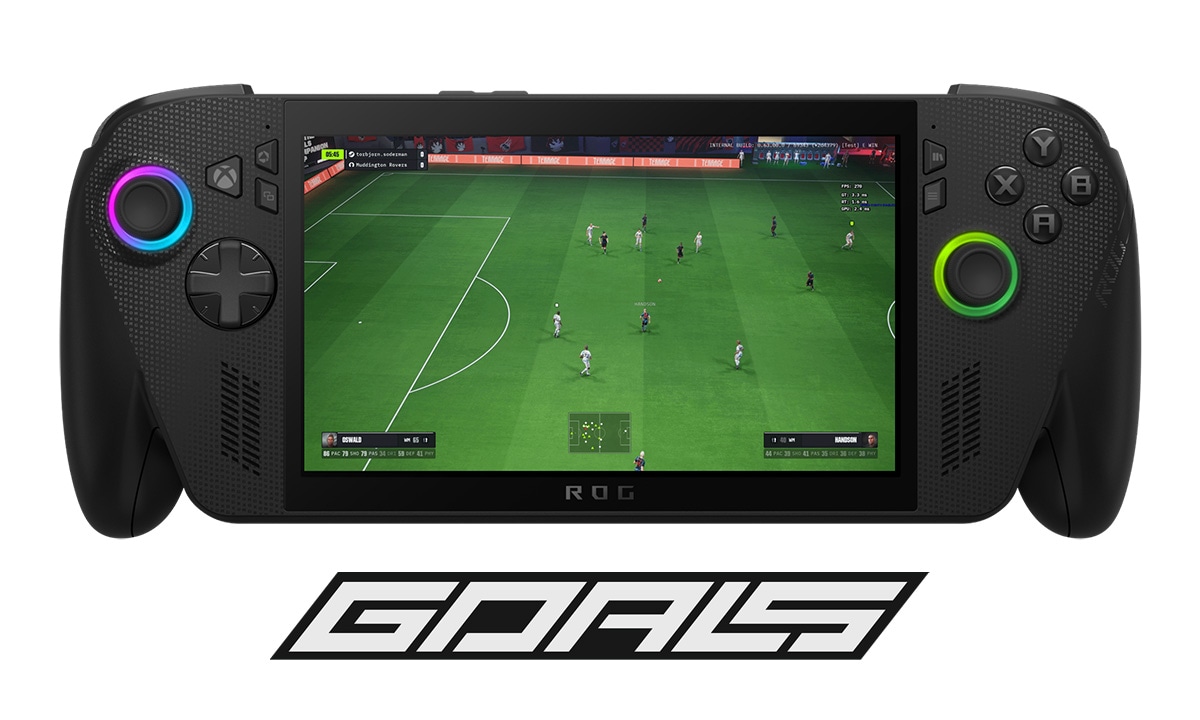 | How GOALS delivers sustained, competitive esports performance on handheld PCs - part 2The second part of how GOALS optimizes AMD Ryzen handheld PC gaming performance using AMD FSR Upscaling and Frame Generation, handcrafted device profiles, football-aware animation budgeting, and battery-aware scalability for sustained play. |
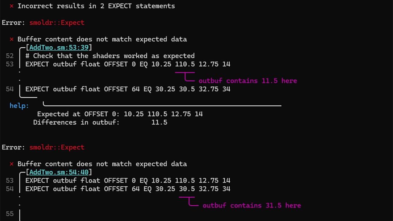 | Enhancing DirectX Testing with AMD SmoldrSmoldr is an open-source command-line tool that runs DirectX 12 HLSL shaders from simple text scripts, letting you compile, create resources and pipelines, and dispatch compute or raytracing workloads without writing C++ code. |
 | AMD and Microsoft partner on DirectX ML, DirectStorage, and developer tools at GDC 2026Microsoft and AMD partnered at GDC to announce powerful new developer technologies for Windows, including DirectStorage 1.4, PIX tools updates, DirectX ML integration, Advanced Shader Delivery, and support for the latest Agility SDK update. |
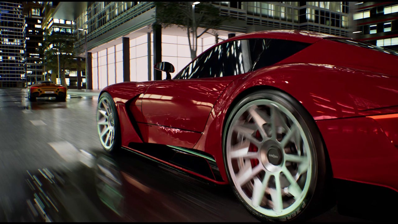
 | Driving the future: frictionless automotive HMI development with Epic Games & AMD Ryzen AI Embedded P100 seriesAt CES 2026 Epic Games and AMD unveiled the Unreal Engine 5 Next‑Gen HMI Experience powered by AMD Ryzen AI Embedded P100 Series, unifying instrument clusters, maps, and apps into a single high‑performance UE5 instance with gaming‑class graphics, and a streamlined developer workflow to deliver customizable, 60 FPS in‑cockpit experiences. |
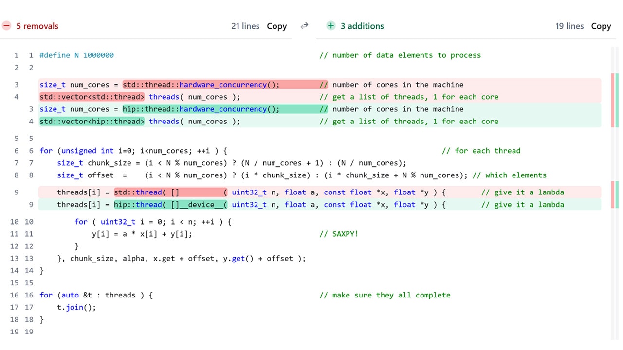 | HIP Threads: GPU power for teams without GPU expertsHIP Threads lets C++ teams eliminate CPU hotspots by running familiar multithreaded code on AMD GPUs, no kernel rewrites or GPU expertise required, delivering real speedups in days. |
| AMD FSR™ Redstone expands with the latest AMD FSR™ SDK 2.1AMD FSR 'Redstone' SDK 2.1 enables developers to integrate FSR features into games with easy-to-use APIs and access to advanced neural rendering technologies. |
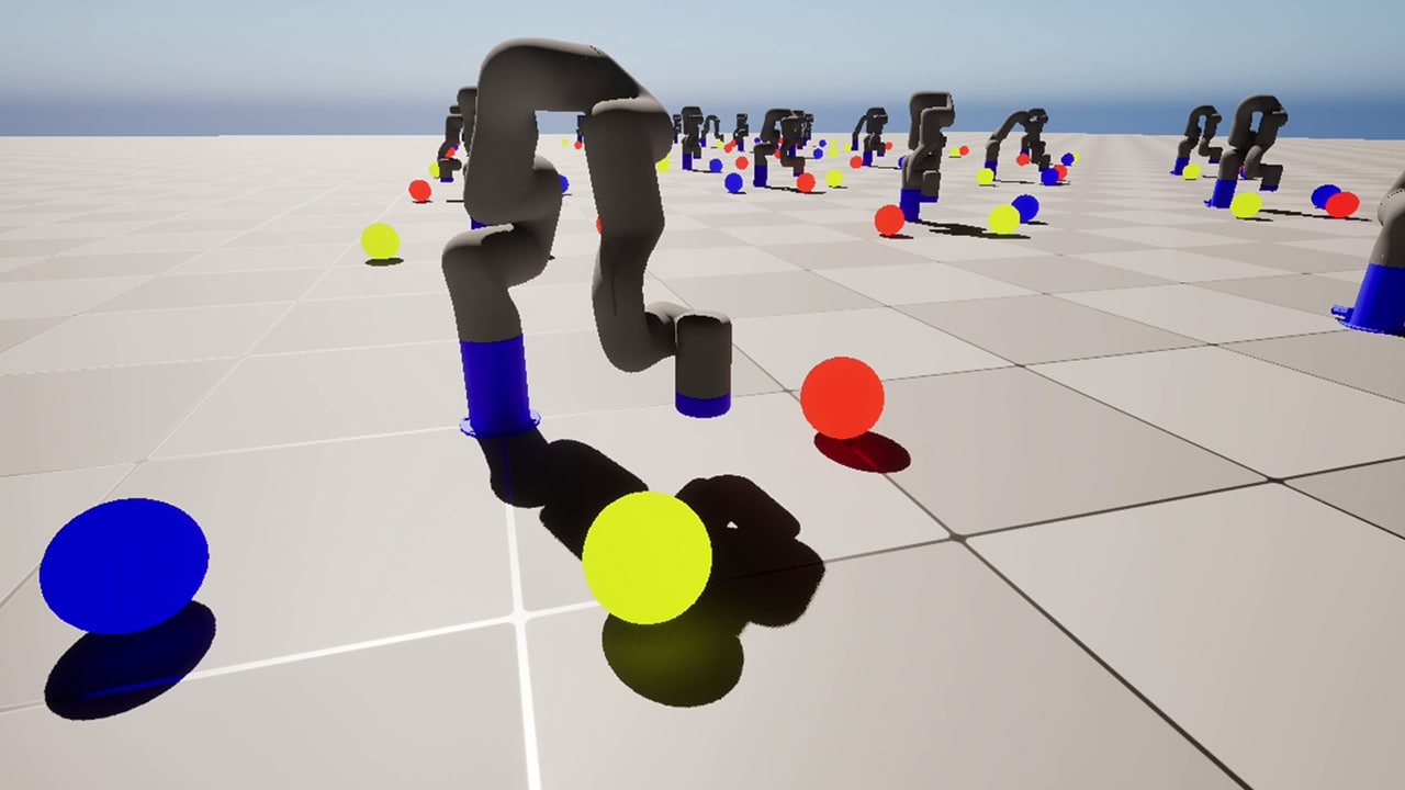 | Training an X-ARM 5 robotic arm with AMD Schola and Unreal EngineTrain a robot arm with reinforcement learning in AMD Schola using Unreal® Engine, progressively increasing task complexity to adapt to changing conditions. |
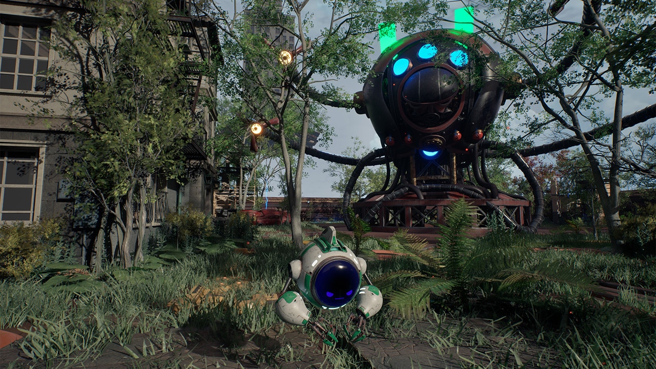 | Announcing AMD Schola v2: Next-generation reinforcement learning for Unreal EngineAMD Schola v2 is a major update to the open-source reinforcement learning plugin for Unreal® Engine 5, offering significant improvements in capabilities, performance, and ease of use for training and deploying AI agents. |
 | Introducing AMD GI-1.2 with multibounce indirect real-time renderingAMD GI-1.2, our real-time Global Illumination solution, is available now as part of the AMD Capsaicin Framework v1.3. |
 | AMD FidelityFX Super Resolution 4 plugin updated for Unreal Engine 5.7Our AMD FSR 4 plugin has been updated to support Unreal® Engine 5.7, empowering you to build expansive, lifelike, and high-performance worlds. |
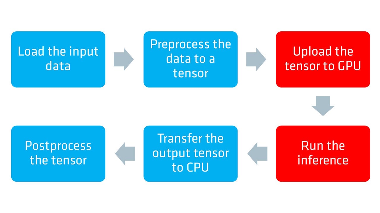 | ONNX and DirectML execution provider guide - part 1Learn how to optimize neural network inference on AMD hardware using the ONNX Runtime with the DirectML execution provider and DirectX 12 in the first part of our guide. |
The AMD FSR SDK 2.1 is the launch vehicle for our ML-based neural rendering technologies. It includes AMD FSR Upscaling, our cutting-edge ML upscaler, plus AMD FSR Frame Generation for smoother gameplay, AMD FSR Ray Regeneration for noise-free ray tracing, and AMD FSR Radiance Caching for efficient real-time global illumination - all using hardware-accelerated features of AMD RDNA™ 4 architecture.
The original AMD FidelityFX SDK v1.1.4 contains our series of optimized, shader-based features aimed at improving rendering quality and performance.
Building something amazing on DirectX®12 or Vulkan®? How about Unreal® Engine?
Obviously you wouldn't dream of shipping without reading our performance and optimization guides for Radeon, Ryzen, or Unreal Engine first!

We aim to provide developer tools that solve your problems.
To achieve this, our tools are built around four key pillars: stability, performance, accuracy, and actionability.