


Finite difference method – Laplacian part 1
The finite difference method is a canonical example of a computational physics stencil discretization commonly used in applications ranging from geophysics (weather and oil & gas) and electromagnetics (semiconductors and astrophysics) to gas dynamics (airflow and plasmas). Stencil codes are identified by an underlying requirement of accessing a local neighborhood of grid points (stencil) in order to evaluate a value at a single grid point, meaning that the performance of the algorithm is strongly tied its memory access pattern. GPUs haven proven to be well-suited for accelerating stencils codes due to the algorithm’s regular structure, high degree of exposed parallelism, and efficient use of the GPU’s high memory bandwidth. In this blog post we will develop a GPU-accelerated stencil code using AMD’s Heterogeneous Interface for Portability (HIP) API, which will give us explicit control over the memory access patterns. Over the course of this development, we will discuss the following concepts:
-
Discretize the Laplacian using the finite difference method
-
Present a straight-forward HIP implementation of the discretization
-
Guide readers on choosing optimization strategies for improving performance of a stencil code
-
Illustrate how to use
rocprofto obtain performance metrics for kernels
Laplacian
The Laplacian \nabla^2 is a differential operator that can describe a variety of physical phenomena using partial differential equations. For example, it can be used to describe propagation of sound waves (wave equation), heat flow (heat equation), as well electrostatic and gravitational potentials (Poisson’s equation). It also has applications within computer vision and mesh generation. See wikipedia to learn more.
As an example of a physical phenomena that can be described by the Laplacian, the animation below is a 2D numerical simulation of the heat equation that shows the transfer of heat from hot regions (raised letters) to cold regions (plane).
|
Initial condition |
Simulation |
|---|---|
|
|
|


In Cartesian coordinates, the Laplacian takes the form of the divergence of a gradient of a scalar field u(x,y,z):
\nabla \cdot \nabla u = \nabla^2 u = \frac{\partial^2u}{\partial x^2} + \frac{\partial^2u}{\partial y^2} + \frac{\partial^2u}{\partial z^2},
where u is a suitably smooth function of the spatial coordinates x, y, and z.
Discretization and host implementation
To discretize the Laplacian, we introduce a grid with n_x \times n_y \times n_z equidistantly-spaced grid points and apply second-order finite difference approximations in each grid direction. For example, the x-derivative is approximated by:
\frac{\partial^2 u}{\partial x^2} \approx \frac{u(x-h_x,y,z) - 2u(x,y,z) + u(x+h_x,y,z)}{h_x^2}
where h_x is the grid spacing in the x-direction (the distance between adjacent grid points in the x-direction). Extending this to three dimensions involves applying this stencil in all spatial directions:
\nabla^2 u(x,y,z) \approx \frac{u(x-h_x,y,z) - 2u(x,y,z) + u(x+h_x,y,z)}{h_x^2}
+ \frac{u(x,y-h_y,z) - 2u(x,y,z) + u(x,y+h_y,z)}{h_y^2}
+ \frac{u(x,y,z-h_z) - 2u(x,y,z) + u(x,y,z+h_z)}{h_z^2}
The following code example demonstrates how to implement the Laplacian stencil in host code:
Copied!
template <typename T>
void laplacian_host(T *h_f, const T *h_u, T hx, T hy, T, hz, int nx, int ny,
int nz) {
#define u(i, j, k) h_u[(i) + (j) * nx  + (k) * nx * ny]
#define f(i, j, k) h_f[(i) + (j) * nx  + (k) * nx * ny]
    // Skip boundary points
    for (k = 1; k < nz - 1; ++k)
        for (j = 1; j < ny - 1; ++j)
            for (i = 1; i < nx - 1; ++i) {
                // Apply stencil approximation of Laplacian to all interior points
                u_xx = ( u(i + 1, j, k) - 2 * u(i, j, k) + u(i - 1, j, k) ) / (hx * hx);
                u_yy = ( u(i, j + 1, k) - 2 * u(i, j, k) + u(i, j - 1, k) ) / (hy * hy);
                u_zz = ( u(i, j, k + 1) - 2 * u(i, j, k) + u(i, j, k - 1) ) / (hz * hz);
                f(i, j, k) = u_xx + u_yy + u_zz;
            }
#undef u
#undef f
}
The host code uses C-preprocessor macros to more easily translate the math notation u(x,y,z) into code: u(i, j, k) – you will learn more about this translation soon. The function laplacian_host takes the input, h_u[], and output, h_f[], and expects them to at least contain nx * ny * nz elements each (the number of grid points in each direction). To prevent memory access violations due to out of bounds errors, the loop bounds exclude the first and last elements in each grid direction. The inner-most loop applies the Laplacian stencil to h_u[] and stores the result in h_f[]. To distinguish host arrays from device arrays, we assign the prefixes h_ (host) and d_ (device). This distinction will become important when we visit the device code.
Data layout
The 3D data is laid out so that grid points in the i-direction are contiguous in memory whereas grid points in the k-direction are strided by nx * ny. This mapping is exemplified by the macro:
Copied!
#define u(i, j, k) h_u[(i) + (j) * nx + (k) * nx * ny]
The parentheses around i, j, and k ensure proper expansion of expressions like u(i, j + 1, k) and so forth.
The figure below shows the Laplacian stencil applied at a grid point pos
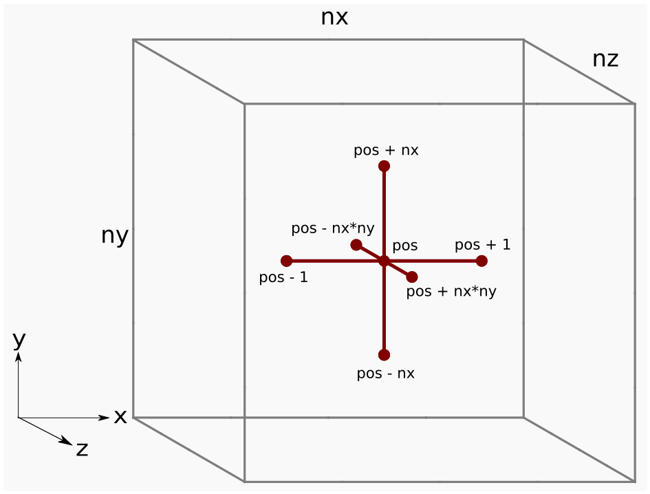
Figure 1: Finite difference stencil in 3D space.
Grid points adjacent to each other in the j and k directions are actually far apart in memory due to the strided data layout. For example, consider when nx = ny = nz = 5:
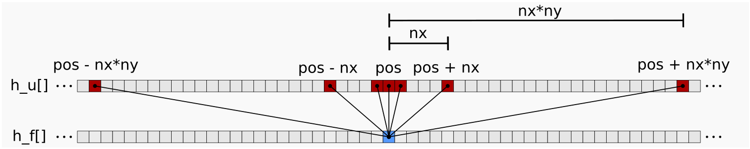
Figure 2: Strided memory space for the central difference stencil. Here we see which entries in the h_u[] array (red) are needed to update the output array h_f[]. Note that these entries are not contiguous.
One of the goals of this blog is to show how to efficiently treat this memory access pattern on AMD GPUs.
HIP implementation
To begin, consider a large cube where nx = ny = nz = 512. We first allocate memory for both the input array d_u and the output array d_f using double precision:
Copied!
// Parameters
using precision = double;
size_t nx = 512, ny = 512, nz = 512; // Cube dimensions

// Grid point spacings
precision hx = 1.0 / (nx - 1), hy = 1.0 / (ny - 1), hz = 1.0 / (nz - 1);

// Input and output arrays
precision *d_u, *d_f;

// Allocate on device
size_t numbytes = nx * ny * nz * sizeof(precision);
hipMalloc((void**)&d_u, numbytes);
hipMalloc((void**)&d_f, numbytes);
The d_u input array is initialized using a quadratic test function that simplifies the task of verifying correctness (not shown for brevity).
The below code snippet presents our initial HIP implementation of the Laplacian:
Copied!
template <typename T>
__global__ void laplacian_kernel(T * f, const T * u, int nx, int ny, int nz, T invhx2, T invhy2, T invhz2, T invhxyz2) {

    int i = threadIdx.x + blockIdx.x * blockDim.x;
    int j = threadIdx.y + blockIdx.y * blockDim.y;
    int k = threadIdx.z + blockIdx.z * blockDim.z;

    // Exit if this thread is on the boundary
    if (i == 0 || i >= nx - 1 ||
        j == 0 || j >= ny - 1 ||
        k == 0 || k >= nz - 1)
        return;

    const int slice = nx * ny;
    size_t pos = i + nx * j + slice * k;

    // Compute the result of the stencil operation
    f[pos] = u[pos] * invhxyz2
           + (u[pos - 1]     + u[pos + 1]) * invhx2
           + (u[pos - nx]    + u[pos + nx]) * invhy2
           + (u[pos - slice] + u[pos + slice]) * invhz2;
}

template <typename T>
void laplacian(T *d_f, T *d_u, int nx, int ny, int nz, int BLK_X, int BLK_Y, int BLK_Z, T hx, T hy, T hz) {

    dim3 block(BLK_X, BLK_Y, BLK_Z);
    dim3 grid((nx - 1) / block.x + 1, (ny - 1) / block.y + 1, (nz - 1) / block.z + 1);
    T invhx2 = (T)1./hx/hx;
    T invhy2 = (T)1./hy/hy;
    T invhz2 = (T)1./hz/hz;
    T invhxyz2 = -2. * (invhx2 + invhy2 + invhz2);

    laplacian_kernel<<<grid, block>>>(d_f, d_u, nx, ny, nz, invhx2, invhy2, invhz2, invhxyz2);
}
The laplacian host function is responsible for launching the device kernel, laplacian_kernel, with a thread block size of BLK_X = 256, BLK_Y = 1, BLK_Z = 1. The current thread block size where BLK_X * BLK_Y * BLK_Z = 256 is a recommended default choice because it maps well to hardware work scheduler, but other choices may perform better. In general, choosing this parameter for performance may be highly dependent on the problem size, kernel implementation, and hardware characteristics of the device. We will discuss this topic in more detail in a future post. Although this kernel implementation supports a 3D block size, the GPU has no concept of 2D and 3D. The possibility of defining 3D groups is provided as a convenience function to the programmer.
The HIP implementation is applicable to any problem size that fits in the GPU memory. For problem sizes that cannot be evenly divided by the thread block size, we introduce additional groups that work on the remainder. These additional thread blocks can have low thread utilization if the remainder is small, i.e., many of the threads map to a region outside the computational domain where there is no work to do. This low thread utilization can negatively impact performance. For the purposes of this blog post we will focus on problem sizes that are evenly divisible by the thread block size. The number of blocks to schedule is determined by the ceiling operation (nx - 1) / block.x + 1, .... As previously explained, it rounds up the number of groups to guarantee that the entire computational domain is covered.
Note the exit condition in the kernel. We return (exit) when a thread is on or outside a boundary because we are computing the finite difference of interior points only. How the kernel exit strategy works in practice is that since a wavefront executes instructions in lockstep, any thread that is on our outside the boundary will be masked off for the remainder kernel. The threads that are masked off will be idle during the execution of an instruction. Let us return to the performance issue with block sizes that do not evenly divide the problem size. If we pick, say nx=258, we would get two thread blocks in the x-direction, but only one of the threads in the second thread block would have work to do.
The main computation,
Copied!
    // Compute the result of the stencil operation
    f[pos] = u[pos] * invhxyz2
           + (u[pos - 1]     + u[pos + 1]) * invhx2
           + (u[pos - nx]    + u[pos + nx]) * invhy2
           + (u[pos - slice] + u[pos + slice]) * invhz2;
accesses the array u multiple times. For each access, the compiler will generate a global load instruction that will access data from global memory unless this data is already present in cache. As we will see, these global load instructions can have significant performance implications.
Compute bound vs memory bound
In order to analyze the performance of our HIP kernel, it is helpful to understand if it is compute or memory bound. Kernels that are compute bound are limited by the throughput of compute units, whereas memory bound kernels are limited by memory bandwidth or memory access latency. To classify our kernel, we investigate its Arithmetic Intensity (AI) with this formula:
\mathrm{AI} = \frac{\mathrm{FLOPs}}{\mathrm{BYTES}}
where \mathrm{FLOPs} refers to the total number of floating-point operations, and \mathrm{BYTES} denotes the main memory traffic. An algorithm is said to be memory bound if \mathrm{AI}\le PF/BW where PF denotes the peak flop rate and BW denotes the peak memory bandwidth. Conversely, an algorithm is said to be compute bound if \mathrm{AI}\ge PF/BW. Note that we are ignoring integer arithmetic and focusing solely on floating-point arithmetic. This analysis of floating-point arithmetic and memory traffic is commonly used for creating a roofline model. For readers interested in learning more about the roofline model, we defer to this wikipedia link and its accompanying references.
In the laplacian_kernel above, each thread performs 10 floating point operations across 7 d_u elements and stores the computation into a single d_f element. However, we will assume ideal conditions with an infinite cache meaning each thread fetches one d_u element, and this element is reused by other threads for the stencil computations. The \mathrm{FLOPs} and \mathrm{BYTES} per thread equals 10 and 2 * sizeof(double) = 16, respectively, so our AI is 0.63. Stencil codes like this generally have small \mathrm{FLOPs} to \mathrm{BYTES} ratios, and it will be even smaller when we lift the infinite cache assumption.
For the remainder of this blog post, let us consider a single Graphics Compute Die (GCD) from an MI250X GPU where PF= 24 TFLOPs/sec and BW= 1.6 TBytes/sec of high bandwidth memory (HBM) bandwidth. The PF/BW ratio is 24 times greater than the approximated AI, clearly classifying our HIP kernel as memory bound as opposed to compute bound. Thus, our optimizations will focus on addressing memory bottlenecks.
Performance
For performance evaluation, we can use effective memory bandwidth as our figure of merit (FOM). Roughly speaking, the effective memory bandwidth is the average rate of data transfer considering the least amount of data that needs to move through the entire memory subsystem: from high-latency off-chip HBM to low-latency registers. The effective memory bandwidth is defined as
Copied!
effective_memory_bandwidth = (theoretical_fetch_size + theoretical_write_size) / average_kernel_execution_time;
To measure the average kernel execution time, we use the function hipEventElapsedTime() (see the accompanying laplacian.cpp for full implementation details). The formula for calculating the theoretical fetch and write sizes (in bytes) of an nx * ny * nz cube are:
Copied!
theoretical_fetch_size = ((nx * ny * nz - 8 - 4 * (nx - 2) - 4 * (ny - 2) - 4 * (nz - 2) ) * sizeof(double);
theoretical_write_size = ((nx - 2) * (ny - 2) * (nz - 2)) * sizeof(double);
Due to the shape of the stencil, the theoretical fetch size accounts for reading all grid points in d_u except for the 8 corners and 12 edges of the cube. In the theoretical write size, only the interior grid points in d_f are written back to memory. These calculations overlook memory access granularity and, again, assume an infinite cache. Thus, they place a lower bound on the actual data movement.
Below are the performance numbers on a single MI250X GCD:
Copied!
$ ./laplacian_dp_kernel1
Kernel: 1
Precision: double
nx,ny,nz = 512, 512, 512
block sizes = 256, 1, 1
Laplacian kernel took: 2.64172 ms, effective memory bandwidth: 808.148 GB/s
For an optimized kernel and sufficiently large workload capable of saturating the device, the effective memory bandwidth should be as close as possible to the peak theoretical HBM bandwidth. Accomplishing this task requires meeting two objectives:
-
reducing excessive memory traffic to HBM to be close as possible to the theoretical limit,
-
Saturating the HBM bandwidth of the device.
Given that a MI250X has a theoretical bandwidth per GCD of 1638.4 GB/s, the baseline kernel achieves about 50 %[1] of the peak theoretical limit. What is the bottleneck preventing further performance? Is it due to excessive data movement or suboptimal memory bandwidth saturation? For instance, excessive data movement could occur if there is poor data reuse when computing the stencil. Maybe some of the neighboring values are brought into cache but evicted by other values, causing cache misses and additional trips to main memory. Failure to saturate memory bandwidth occurs when there are not enough memory requests in flight during the life time of the kernel. There could be many reasons for this problem in general. Maybe each wave requests very little data and there are not enough waves that can run concurrently on each CU due to resource limitations. Another possibility is that some of the waves are stalled and ineligible for issuing memory instructions to because they are waiting on data dependencies. To understand what the bottleneck is and address it, we need to collect performance counter data.
To this end, we use the AMD ROCm™ profiler (rocprof) to capture three important metrics:
Copied!
FETCH_SIZE : The total kilobytes fetched from the video memory. This is
             measured with all extra fetches and any cache or memory effects
             taken into account.
WRITE_SIZE : The total kilobytes written to the video memory. This is measured
             with all extra fetches and any cache or memory effects taken
             into account.
L2CacheHit : The percentage of fetch, write, atomic, and other instructions that
             hit the data in L2 cache. Value range: 0% (no hit) to 100% (optimal).
Note that the sum of FETCH_SIZE and WRITE_SUM may not truly represent all memory traffic. Nonetheless these metrics can certainly provide greater insight into the design of the HIP kernels. Additional metrics can be queried from rocprof (see rocprof --list-basic and rocprof --list-derived for options). rocprof allows us to organize our requests within ascii text files. For example, in the included work we use rocprof_input.txt:
Copied!
pmc: FETCH_SIZE
pmc: WRITE_SIZE
pmc: L2CacheHit
kernel: laplacian_kernel
which will capture the performance counters (pmc) FETCH_SIZE, WRITE_SIZE, and L2CacheHit for the listed kernels. We can run this against our executables using the command
Copied!
$ rocprof -i rocprof_input.txt -o rocprof_output.csv laplacian_dp_kernel
which will generate a rocprof_output.csv file containing the requested metrics for each kernel launch. For more information on rocprof we defer all interested readers to the ROCm™ Profiler documentation.
The closer FETCH_SIZE and WRITE_SIZE are to theoretical_fetch_size and theoretical_write_size, the better our HIP kernel is likely to perform. An L2CacheHit closer to 100% is another indicator that our kernel is optimal. The table below compares the above three rocprof metrics:
|
FETCH_SIZE (GB) |
WRITE_SIZE (GB) |
Fetch efficiency (%) |
Write efficiency (%) |
L2CacheHit (%) |
|
|---|---|---|---|---|---|
|
Theoretical |
1.074 |
1.061 |
– |
– |
– |
|
Kernel 1 |
2.014 |
1.064 |
53.3 |
99.7 |
65.0 |
The 65% L2CacheHit rate alone doesn’t offer much insight. While the WRITE_SIZE metric matches its theoretical estimate, the FETCH_SIZE is nearly doubled. This observation tells us that about 50 % of the stencil is reused. If we can improve the stencil reuse to 100 %, the FETCH_SIZE would reduce by over 0.9 GB and in turn reduce the total memory traffic by 31 %. This reduction could potentially translate into a 1.44x speedup of the kernel execution time, assuming HBM bandwidth saturation remains the same. Therefore, a more realistic target for effective memory bandwidth would be around 808.148 GB/s * 1.44 = 1165 GB/s, which is about 71 %[1] of the peak theoretical HBM bandwidth of 1638.4 GB/s per GCD.
There are several different approaches to optimizing finite difference kernels in general. In the next post, we will explain and discuss a few optimizations that one can apply to reduce excess memory traffic and reach the new effect memory bandwidth target.
Conclusion
This concludes the first part of developing and optimizing a Laplacian kernel using HIP. Before beginning any optimization work, it is important to collect performance measurements to establish a baseline and identify the performance bottleneck. In this work, we have determined that the baseline kernel is memory bandwidth limited due to its arithmetic intensity. We also found that the kernel loads significantly more data from the global memory space compared to our estimates. These conditions tell us that reducing the excess memory load will have an impact on performance. In part two of this series we will introduce optimization techniques aimed at reducing global memory data movement which are valuable not only for stencil kernels, but also for other bandwidth limited kernels that use a regular, non-contiguous memory access patterns.
If you have any questions or comments, please reach out to us on GitHub Discussions